Machine Learning and Deep Learning in Finance: A Complete Guide to 10 Models

Most articles about machine learning in finance show a model, report a number, and stop. Stopping there is the problem, because a number on its own never answers the question a desk actually asks, which is whether something simpler would have done the same job for nothing.

Ten models run below on real market data. Five from the classical side, decision trees through Lasso, and five neural networks, feed forward through autoencoders. Each one is pointed at a task that suits its structure rather than at whatever produces the prettiest curve. Every split is by date. Every data source is free.

Section 5 then does the part that usually gets skipped. It scores the two sequence models and the convolutional net against baselines that cost nothing, on the identical rows, and all three lose. That result stays in.

Code first, since that is what most people want. Both repositories run top to bottom on free data, and every chart in this article is reproduced by the scripts that made it. Classical models are here and the neural networks and the baselines are here.

Watch it built, end to end

Video below takes the same ideas the whole way: 94 firm characteristics into a neural network, predictions ranked into a long short book, then wired to the Interactive Brokers API so the model places its own orders rather than printing a backtest. Subtitles in English, Portuguese and Spanish.

1. Glossary, so nothing later needs unpacking

1.1 Supervised, unsupervised, and why it matters here

A supervised model gets features and an answer, and learns the map between them. Eight of the ten below are supervised. Unsupervised models get features and no answer, and are asked to describe structure instead of predicting it. PCA and the autoencoder are the two, and they turn out to be the most reliable pair in the article, which is not a coincidence. Describing structure that genuinely exists is a far easier problem than forecasting a return.

1.2 Splitting by date, and why random splitting is a lie

Shuffling rows and holding out 20% is standard in machine learning and invalid in finance. Prices are autocorrelated, so a shuffled test set contains days that sit between two training days, and the model interpolates rather than forecasts. Every result here splits at a date: everything before it trains, everything after it is scored. Section 4.1 is the single exception, and it says so, because fitting a surface quoted at one instant carries no time ordering to respect.

1.3 Survivorship, the bias that flatters everything

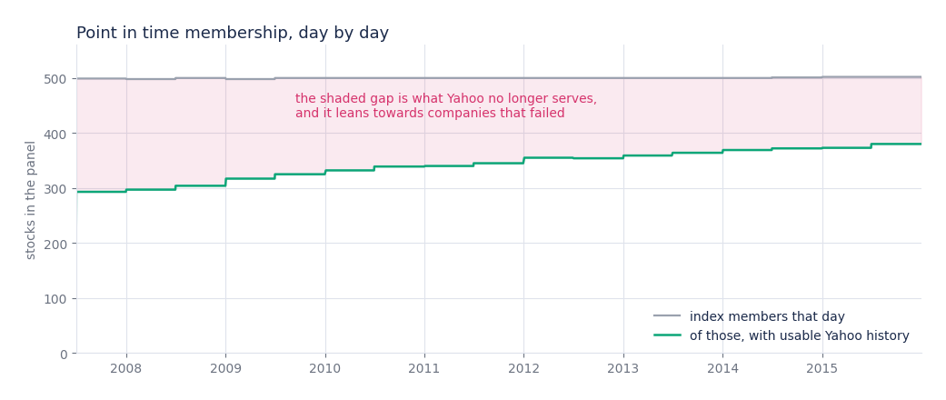
Downloading today's S&P 500 list and running it back to 2007 tests a strategy on companies already known to have survived. Membership here is rebuilt point in time from index history, so a company that was in the index in 2011 and gone by 2015 is present until it left and absent after. That yields 640 tickers with usable data and a median of 342 members on any given day.

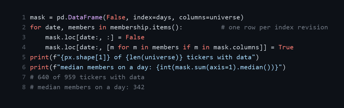
Every feature below is computed through that mask, so a company contributes rows only on the days it was actually in the index. Removing the mask and using today's list instead lifts the headline numbers, which is exactly why so many published backtests look better than they are.

1.4 How to read the numbers

Classification models are scored with AUC, where 0.50 is a coin flip. Forecasts are scored with correlation against what actually happened, and with RMSE in the units of the target. Trading results are reported as return per day of a long short book with a t statistic, before costs. No figure below has transaction costs in it, and none of it is a backtest with money in it.

2. Trees, and a published strategy rebuilt

Sections 2.1 to 2.3 rebuild the tree based half of Krauss, Do and Huck (2017), Deep neural networks, gradient boosted trees, random forests: Statistical arbitrage on the S&P 500, on free data. Same construction: train on 750 days, trade the next 250, step forward and refit. Features are cumulative returns over 1 to 20 days and then 40, 60 up to 240, standardised across the cross section of each day. Target is whether a stock beats the median stock tomorrow. Trade only the extremes, long the ten highest probabilities and short the ten lowest.

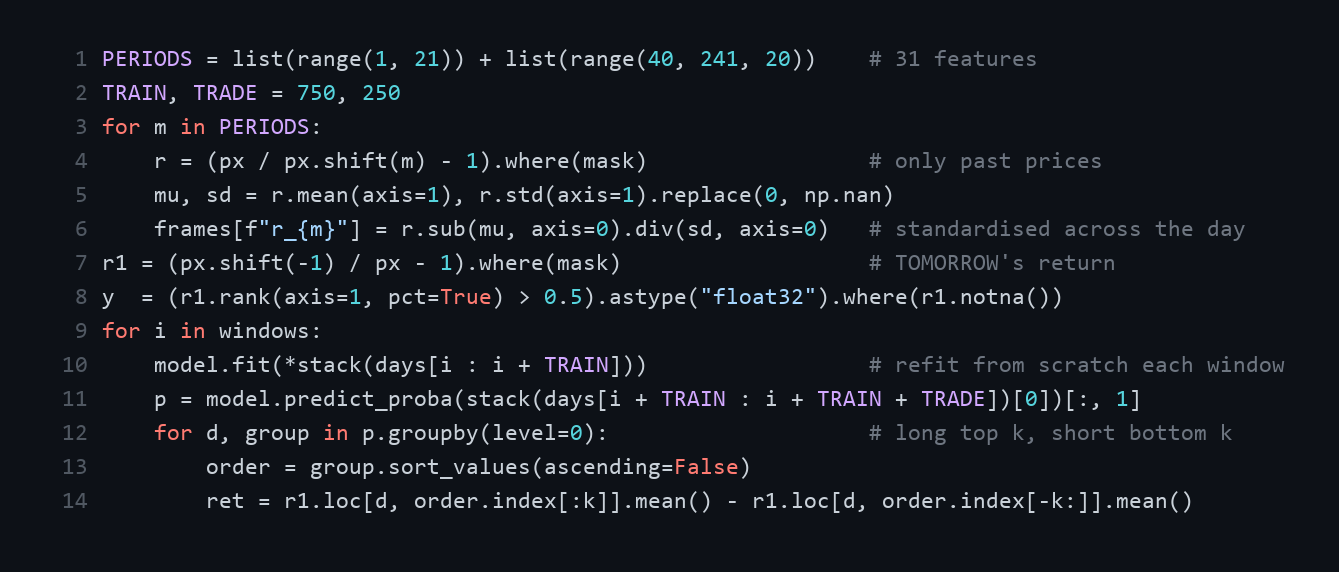
Standardising across the cross section of each day is what makes the target relative. A model cannot win by learning that markets drift upward, because on every single day half the names are labelled one and half are labelled zero.

2.1 Decision tree

One tree, grown alone, splitting on whichever threshold removes the most uncertainty until each leaf holds a rule you can read in English. Accuracy sits below every ensemble in this article, and credit committees sign it anyway, because a regulator asking why an application was declined wants a reason code rather than a SHAP plot.

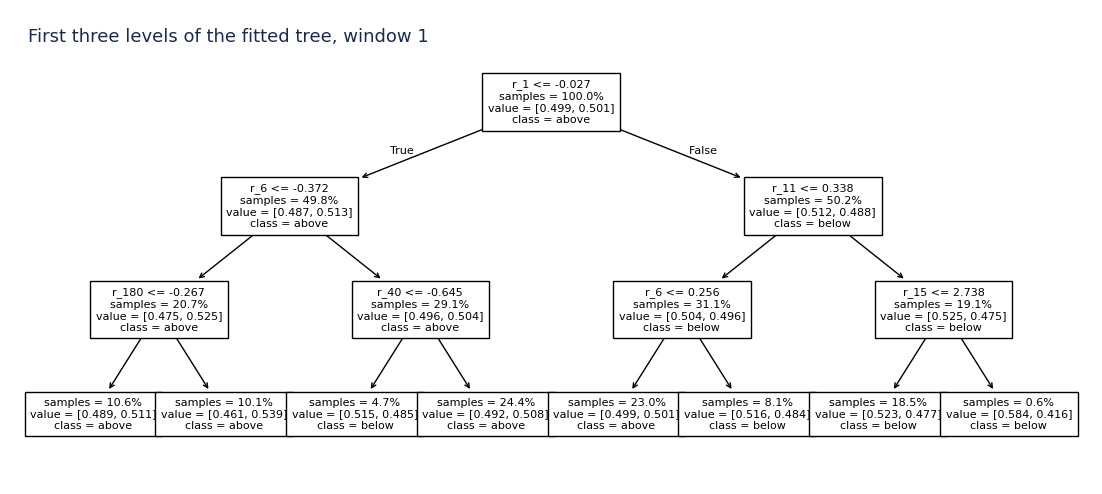
Out of sample it returns 0.055% a day with a t statistic of 2.02. Same sign as the paper, a fraction of the size.

2.2 Random forest

Hundreds of trees, each grown on its own bootstrap sample and allowed to see only a random subset of columns at every split. Answer is the vote. That double randomisation decorrelates the trees so averaging cancels variance instead of compounding it.

Out of sample: 0.160% a day, t = 4.80. Paper reports 0.43% a day at t = 14.93 on its own period, so this reproduces at roughly 37% of the published effect.

2.3 Gradient boosting

Trees built one after another, each fitting the error the ensemble has left rather than the target itself, with the second derivative of the loss sizing how far each leaf may move.

Out of sample: 0.123% a day, t = 3.36, about 33% of the 0.37% the paper reports for the same family.

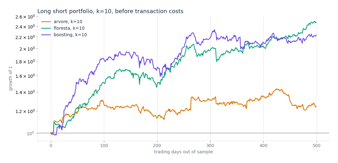
Two facts hold at once here, and holding them together is the whole skill. AUC is 0.51 against a coin flip's 0.50, which is nearly nothing. And the book still earns a real spread, because it only ever touches the two ends of the ranking, where the thin edge concentrates. A model can be almost useless as a classifier and still be tradeable as a sort.

2.4 Why AUC near 0.51 still pays

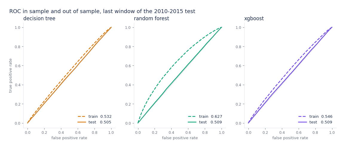
Ranking accuracy of 0.51 sounds like nothing, and it is nothing across the middle of the distribution. A long short book never touches the middle. It takes the ten highest and the ten lowest probabilities of each day, where the edge concentrates, and leaves the other 320 names alone. Same model, judged as a classifier, is close to useless; judged as a sort, it is tradeable.

2.5 What happens when the same code runs to 2025

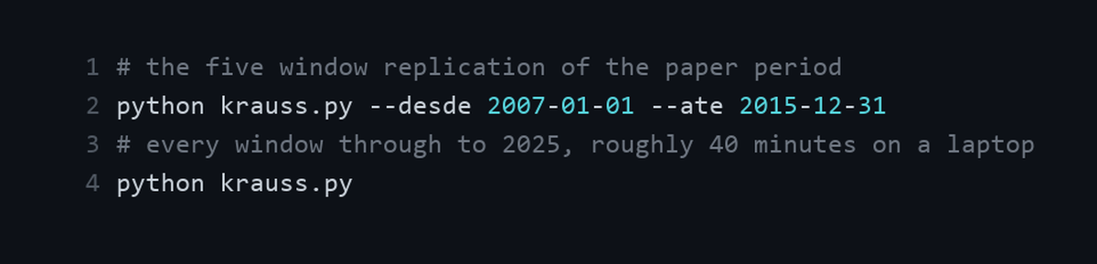
Same code, wider period. Effect decays hard. Roughly a sixth of a percent a day before costs on the years the paper covers, and roughly a thirtieth of that by 2025. That decay is the most useful single number in this article, because it is what a strategy looks like after a decade of being published, read and competed away.

A peer reviewed, widely cited strategy delivers roughly a sixth of a percent a day before costs on the period it was written about, and roughly a thirtieth of that by 2025. Any backtest reporting far more, on free daily data and price features alone, is worth reading twice.

3. Unsupervised and sparse

3.1 PCA on the Treasury curve

PCA is not a predictor. It rotates correlated variables into uncorrelated ones ordered by how much variance each carries. Run it on the daily changes of ten Treasury maturities, never the levels, and the first three components arrive with shapes that have names.

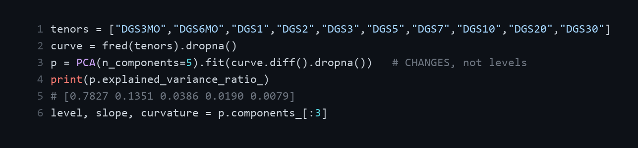
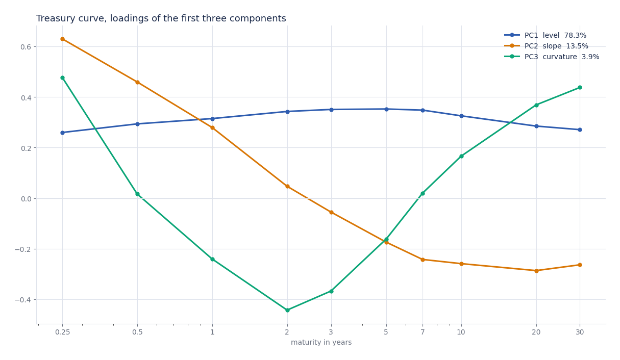
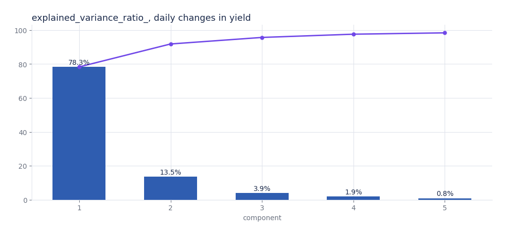
95.64% of daily variation in three components. Cover three risks instead of ten that move together, and the components hold their shape across regimes.

3.2 Lasso

Linear regression carrying a penalty on the size of its own coefficients. L1 puts corners on the constraint region, so coefficients land on exactly zero and variables drop out during the fit rather than after it. With fifty candidate signals and twenty years of data, ordinary least squares fits noise and reports it as skill.

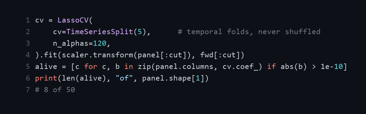
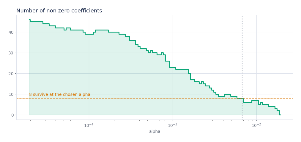
Out of sample R² of 0.0908 on 21 day returns, against −0.0080 for predicting the mean. Small, and pointed in the right direction.

4. Neural networks

Trees stop somewhere. A network only earns its cost when the data has a shape a table cannot hold: a smile across strikes, a sequence with memory, a picture, a cross section with hidden factors. Five architectures, each on the job it was invented for.

4.1 Feed forward, on the volatility surface

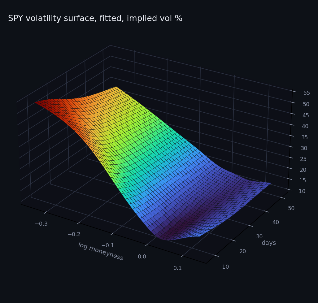
Plainest architecture there is. Every input reaches every unit of the next layer, each unit sums what arrives, bends it through a non linear function and passes it on. No memory between calls. Feed it log moneyness and maturity, get one number back, and that number is a point on an implied volatility surface.

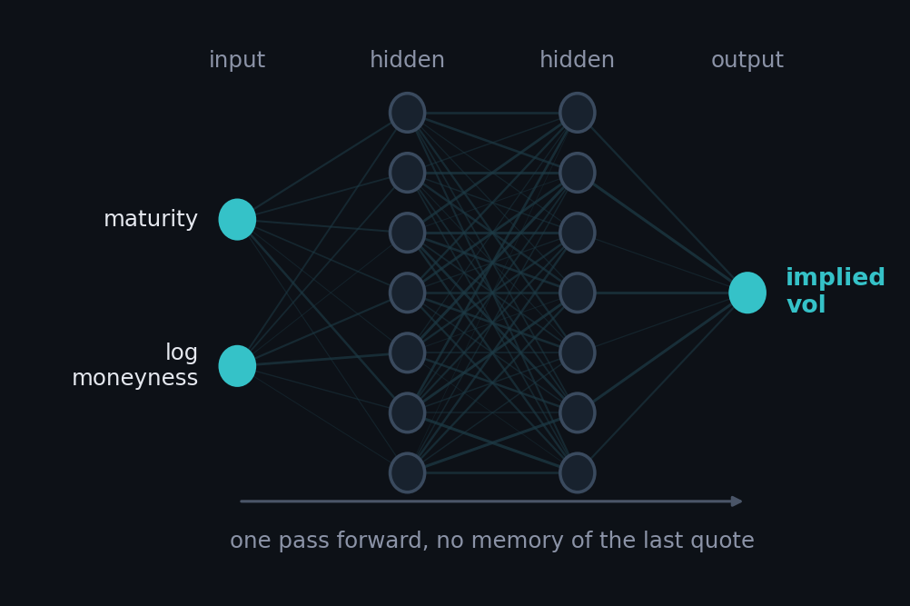
Fitted on 998 live SPY quotes, out of the money only, because a call and a put on one strike carry different quoted vols and feeding both teaches the net to average two different things. Held out error settles at 0.251 volatility points, inside the bid ask spread on most of the chain.

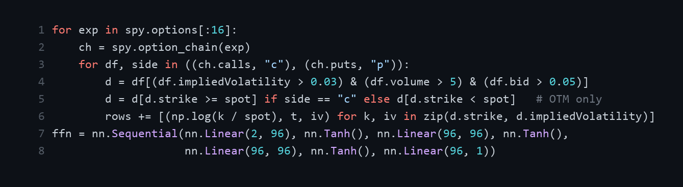
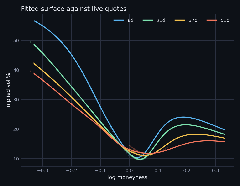
Honest caveat, and section 5 does not reach this one: interpolating a surface is not forecasting. A spline or an SVI fit would do the same job and respect no arbitrage conditions, which this network does not.

4.2 Recurrent, on volatility that remembers

One addition changes everything. A hidden state travels from step to step, so the network reads a sequence in order and what it saw yesterday still colours today. An LSTM wraps that state in gates deciding what to keep and what to drop, which is how forty days survive instead of fading after five.

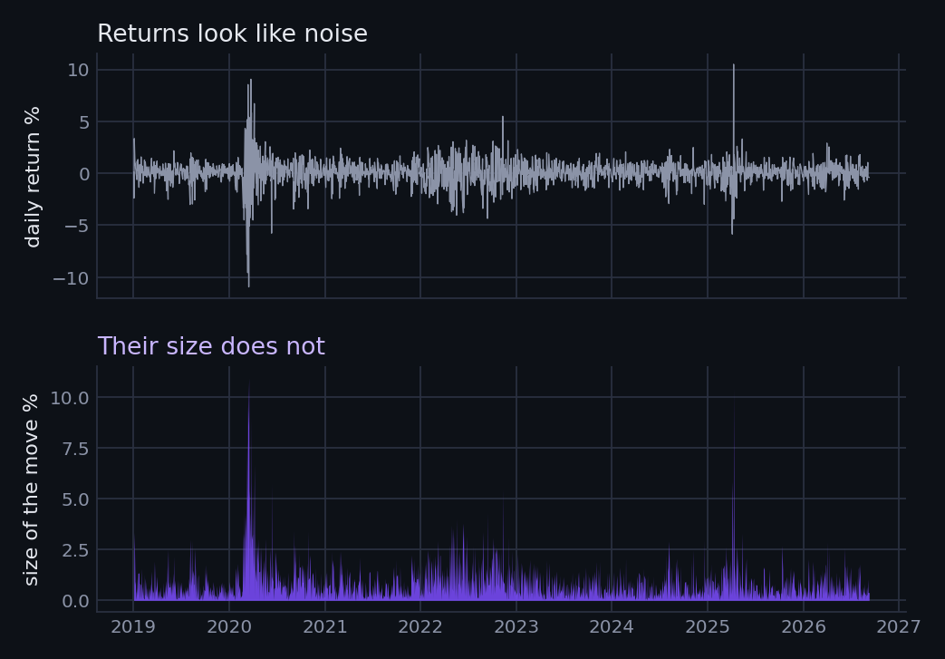
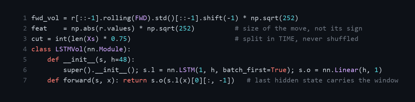
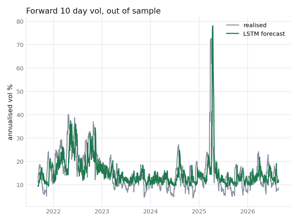
Trained to 7 September 2021 and pushed forward on 4,978 windows, correlation with realised volatility over the next ten days comes to 0.457, RMSE 7.74 volatility points.

4.3 Convolutional, reading a chart as a picture

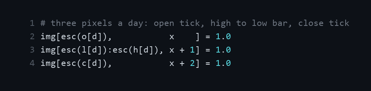
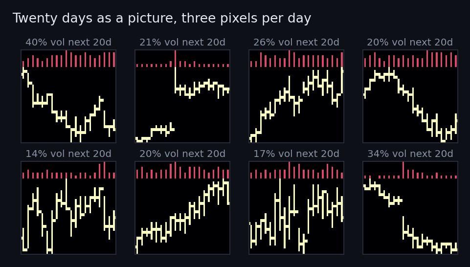
Convolution slides a small filter across an input and asks the same question at every position. Following Jiang, Kelly and Xiu (2023), (Re-)Imag(in)ing Price Trends, twenty trading days are rendered as a bar chart image, three pixels per day, and prices are rescaled inside each window so level disappears and only shape survives.

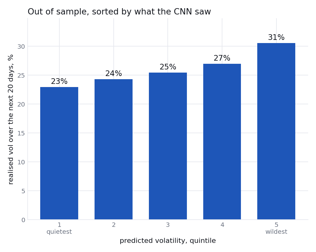
Ask it which way the name goes and a coin does as well: four runs of identical code returned quintile spreads of 0.19, 0.18, 0.01 and 0.16 percentage points. Spread that moves that much between runs is not a result. Ask how much it moves and the picture answers, with the quietest quintile realising 22.9% volatility against 30.6% for the wildest.

4.4 Transformer, and where attention actually pays

Attention replaces the chain. Every day in the window looks at every other day at once, and a learned score sets the weight each one carries. Query, key and value do the work. Same mechanism sits under every large language model.

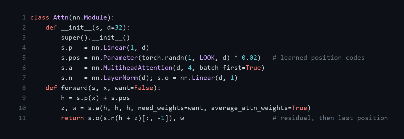
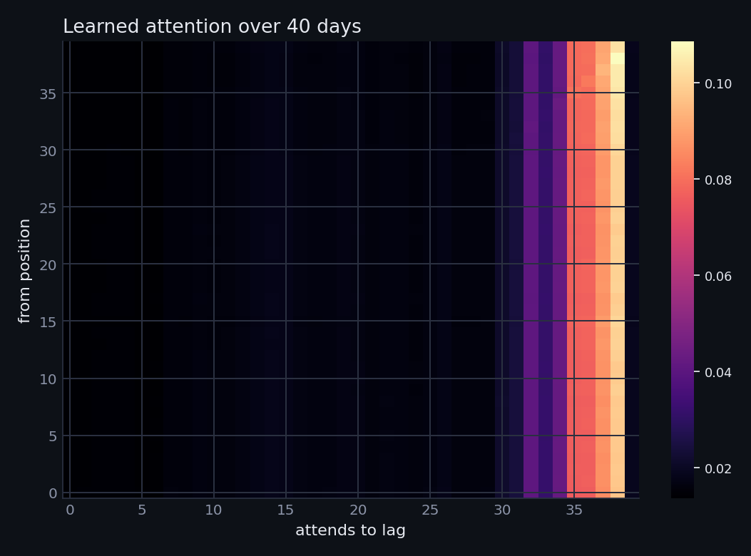
On the same volatility target: correlation 0.446, RMSE 7.81. Read alone that looks like a narrow loss to the LSTM. Section 5 retrains both five times and shows the gap sits inside the noise.

Forty daily numbers is a toy sequence for attention. Text is where transformers genuinely pay in finance: FinBERT and its descendants read filings, earnings calls and news into a sentiment score, and the attention map shows which sentence moved it. Nothing of that kind was trained here.

4.5 Autoencoder, and what survives a squeeze

An autoencoder learns by rebuilding its own input. Daily returns of 45 names go in, get squeezed through three units, and come back out. Nothing supervises it, so those three have to carry whatever is common across the cross section.

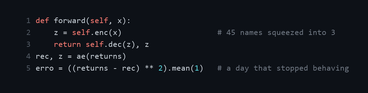
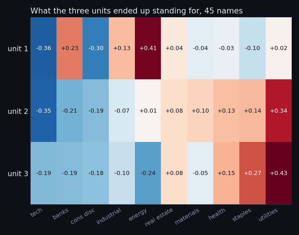
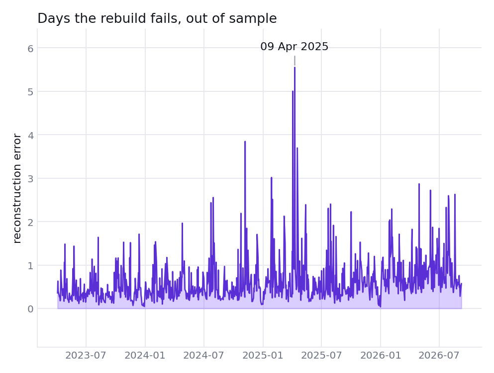
35.0% of the variance of 45 names through three units, out of sample over 3,440 days. Two uses fall out of that. What the units hold is a factor set for hedging and for residuals in statistical arbitrage. What the rebuild misses is a day the cross section stopped behaving, and out of sample the worst one lands on 9 April 2025.

5. Baselines that beat them

Every number above was scored on its own, which answers whether a model learned something and leaves open whether anything simpler would have done as well. Below, each baseline runs on the identical windows, rows and date split.

5.1 Volatility: four fitted coefficients beat both networks

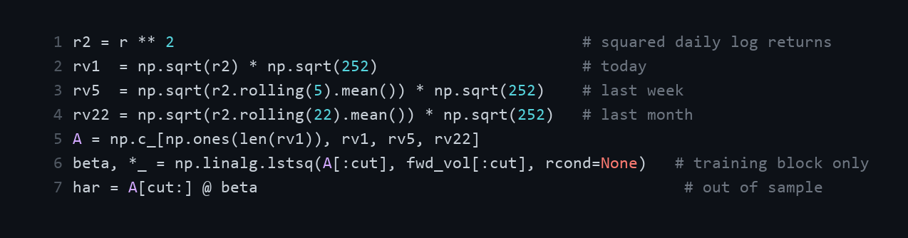
Three baselines for the ten day forward volatility target of sections 4.2 and 4.4. Persistence takes the realised volatility of the last ten days and predicts it continues. EWMA is the RiskMetrics filter at decay 0.94. HAR-RV, from Corsi (2009), regresses forward volatility on daily, weekly and monthly realised volatility. Four coefficients, fitted on the training block, frozen.

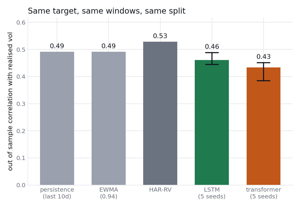
Persistence and EWMA both reach 0.49. HAR-RV reaches 0.53. Both networks were then retrained five times from different seeds: LSTM averaged 0.46, transformer 0.43.

Reading is uncomfortable and clear. Ten day volatility on SPY is forecastable, and on forty daily absolute returns a linear model with the right three features extracts more of it than a recurrent cell or an attention head, at a fraction of the cost. Sections 4.2 and 4.4 stand as demonstrations of how each architecture reads a sequence. As forecasts they lose to the boring thing.

5.2 LSTM against transformer, read against the seeds

Seed by seed, LSTM minus transformer: 0.000, 0.013, 0.015, 0.104, 0.006. Three of five gaps sit inside 0.015, one is zero, and the mean is carried almost entirely by a single transformer seed that collapsed to 0.384. Fair verdict on a sequence this short is that neither separates, and the transformer is the less stable of the two. Any article declaring a winner on one run of each is declaring a winner on noise.

5.3 The number the picture was denied

Section 4.3 rescales prices inside each window so only shape survives. Right design for a direction question, and for a magnitude question it throws away the most useful number available, which is how much the name moved over those same twenty days. Scoring that single number on the identical 38,250 out of sample rows gives correlation 0.513 against 0.225 for the network.

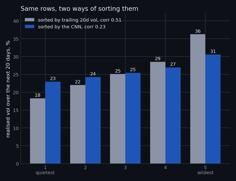
Convolution did recover a real signal from shape. Number it never saw carries more than twice as much.

6. Everything on one line

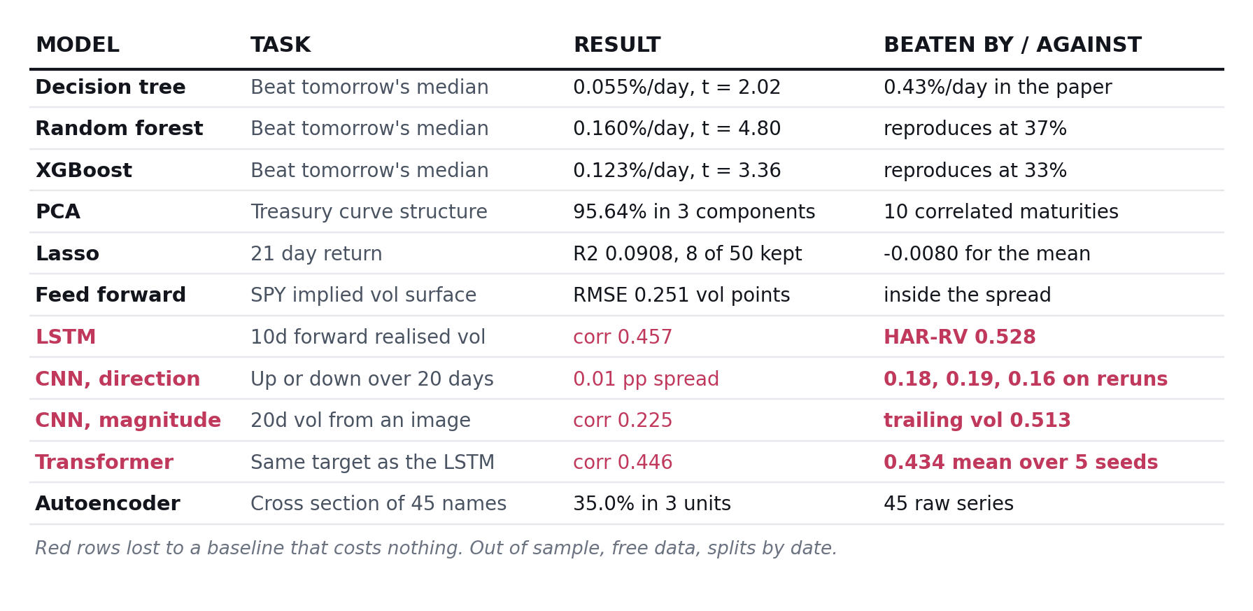
Matching the architecture to the shape of the data is half the lesson. A static map got a feed forward net and landed inside the spread. Correlated maturities got PCA and gave up level, slope and curvature. A cross section got an autoencoder and gave up its sectors.

Other half costs more to learn. Volatility is forecastable, and here a four coefficient linear model forecasts it better than either sequence network, while the single number the CNN was denied forecasts it better than the CNN. Deep learning earns its cost when the input holds structure a linear model cannot: a cross section, an order book, a filing. On forty daily numbers it did not.

7. Limitations

No transaction costs anywhere. No commission, spread, slippage, borrow or impact. Quintile ladders are sorts rather than strategies, and nothing here is a backtest with money in it.

Forty five names is a sample and not a market, all of them alive today, which is survivorship bias by construction in sections 4.3 and 4.5. Volatility windows overlap heavily, so two consecutive labels share nine of their ten days and 4,978 windows are nowhere near 4,978 independent observations. Headline figures come from single runs with a fixed seed, except where section 5 reports five. Adjusted prices carry today's split and dividend factors back through history, which is standard practice and still not strictly point in time.

None of that makes the exercise pointless. It makes it a set of worked examples, each showing which architecture suits which shape of data, with the failures kept in view beside the successes.

Where to go next

Repositories are linked at the top, and both run on free data with no API keys. Longer write ups, with every step, every chart and the limitations in full, live at machine learning for finance and deep learning for finance.