
Decision trees, random forests and XGBoost reproducing a published statistical arbitrage paper on the S&P 500, then PCA on the Treasury curve and Lasso on a macro panel. Free data throughout, point in time index membership, a sliding window that refits five times, and a look at how much of the published edge is left by 2025.
Ninety four firm characteristics feed a neural network with three hidden layers, trained on expanding windows so that validation never sees the future. Predictions rank every stock, then the top decile is bought and the bottom decile sold. Model selection runs on the information coefficient rather than mean squared error, which holds up better on limited data. Method comes from Gu, Kelly and Xiu (2020), Empirical Asset Pricing via Machine Learning, rebuilt here on free data instead of the 30,000 stocks and 920 features of the original. Last step connects the book to the Interactive Brokers API through a Python script, so the strategy places its own long short orders rather than printing a backtest. Code and notebook are on GitHub.
I post the models as I build them, the changes I make to them, and the results that did not work. Shorter than these write ups, and there are a lot more of them.
Follow me on X


One notebook, five models, real data. Every block below is a cell, in the order it runs, so the page and the notebook are the same thing written out. Nothing is simulated and no seed is standing in for a result.
Steps 4 to 7 are a replication rather than an invention. They rebuild the tree based half of Krauss, Do and Huck (2017), a statistical arbitrage paper on the S&P 500, on free data, and then check how much of it survives on years the paper never saw. Steps 8 and 9 are separate: PCA on the Treasury curve, and Lasso on a wide factor panel.
Two ways to use it, and neither is worse than the other.
Follow the steps on this page. Every block is explained before it appears, with the charts it produces and what the numbers mean, so you can read it straight through or copy the blocks in order and build the thing yourself. Step 0 installs everything and imports everything, so no later block reaches for something quietly imported three sections earlier.
Or take the notebook. Same cells, same order, same numbers, ready to run top to bottom. It is further down this page, after the last step, and the only file you need.
Treat these as worked examples, sized to be read in one sitting and run on a laptop. They are here to show the method honestly, not to be lifted into production. For serious work the right next step is the literature, and a good starting point is five machine learning papers that reshaped quant finance.
Read the limitations before trusting any number here. Survivorship is reduced and not eliminated, there are no transaction costs anywhere, the replication covers five windows rather than the paper's twenty three years, and it stops in 2015 on purpose.
Split by date, never at random. Shuffling a price panel lets a model learn from next week while it is fitted on this week. Every split here is temporal. Steps 5 to 7 go further and refit on a sliding window, training on 750 days and scoring only on the 250 that follow, so no model is ever measured on a day that existed when it was fitted.
Score against the naive alternative. An accuracy figure means nothing on its own. The target here is balanced 50/50 by construction, so guessing scores 0.50, and the published result the replication is aimed at gives a second yardstick with a number attached.
Everything the notebook needs, in one place, before anything runs. No API key is required at any point: prices come from Yahoo Finance through yfinance, rates and macro from the public FRED CSV endpoint, and index membership from the Wikipedia API.
Worth knowing that yfinance is an unofficial wrapper around endpoints Yahoo can
throttle or change without notice, which makes it the fragile link in the chain.
Install
pip install yfinance pandas numpy scikit-learn xgboost matplotlib requests lxml pyarrowImports and settings, used by every block that follows
import io, json, time
from pathlib import Path

import numpy as np
import pandas as pd
import requests
import yfinance as yf
import matplotlib.pyplot as plt

from sklearn.tree import DecisionTreeClassifier
from sklearn.ensemble import RandomForestClassifier
from sklearn.decomposition import PCA
from sklearn.linear_model import LassoCV, lasso_path
from sklearn.preprocessing import StandardScaler
from sklearn.model_selection import TimeSeriesSplit
from sklearn.metrics import roc_auc_score, log_loss, r2_score
import xgboost as xgb

START, END  = "2007-01-01", "2015-12-31"   # the overlap with the paper's sample
TRAIN, TRADE = 750, 250                    # sliding window, in trading days
PERIODS = list(range(1, 21)) + list(range(40, 241, 20))   # 31 lookbacks
HEADERS  = {"User-Agent": "Mozilla/5.0 (research)"}
WIKI_API = "https://en.wikipedia.org/w/api.php"FRED through its public CSV endpoint. Steps 8 and 9 pull the Treasury curve and six macro series through it, and it needs no API key, only a URL.
def fred(series):
    """FRED through the public CSV endpoint, no API key required."""
    out = {}
    for s in series:
        r = requests.get("https://fred.stlouisfed.org/graph/fredgraph.csv",
                         params={"id": s}, timeout=90)
        r.raise_for_status()
        d = pd.read_csv(io.StringIO(r.text))
        d.columns = ["date", s]
        d["date"] = pd.to_datetime(d["date"])
        out[s] = pd.to_numeric(d.set_index("date")[s], errors="coerce")
    return pd.DataFrame(out)
Downloading today's S&P 500 list and running it back to 2007 is the most common way to produce a flattering backtest. Every company that went bankrupt, was acquired or simply fell out of the index is absent, so the sample consists entirely of survivors, and a model is then asked to rank companies that were, by construction, the ones that made it.
Point in time membership is the fix. Wikipedia's list of S&P 500 companies keeps a complete revision history, so the constituents as they actually stood on any past date can be read back from the revision live at that date. Taking a snapshot every six months from 2007 onward gives the real membership through time, including names that no longer exist.
Wikipedia needs to be treated politely, with a real user agent and a throttle between requests. Skipping that gets you rate limited, which returns something that is not JSON, so the retry loop below is doing real work rather than being defensive for its own sake.
Slow cell, and cached to disk afterwards
CACHE = Path("membership.json")

def members_on(date):
    p = {"action": "query", "prop": "revisions", "titles": "List of S&P 500 companies",
         "rvlimit": 1, "rvstart": f"{date}T00:00:00Z", "rvdir": "older",
         "rvprop": "ids|timestamp", "format": "json", "formatversion": 2}
    for attempt in range(4):
        resp = requests.get(WIKI_API, params=p, headers=HEADERS, timeout=90)
        try:
            j = resp.json(); break
        except ValueError:                       # rate limited, back off
            time.sleep(3 * (attempt + 1))
    else:
        return []
    rev = j["query"]["pages"][0].get("revisions")
    if not rev:
        return []
    html = requests.get("https://en.wikipedia.org/w/index.php",
                        params={"oldid": rev[0]["revid"]}, headers=HEADERS, timeout=90).text
    try:
        big = [t for t in pd.read_html(io.StringIO(html)) if t.shape[0] > 300]
    except ValueError:
        return []
    if not big:
        return []
    col = [c for c in big[0].columns if str(c).lower().startswith(("symbol", "ticker"))]
    if not col:
        return []
    tick = (big[0][col[0]].astype("string").fillna("").str.strip().str.upper()
            .str.replace(".", "-", regex=False))          # BRK.B -> BRK-B, Yahoo format
    return sorted({x for x in tick.tolist()               # fillna: some revisions carry NaN
                   if isinstance(x, str) and x.isascii()
                   and 1 <= len(x) <= 6 and x.replace("-", "").isalpha()})


snapshots = json.loads(CACHE.read_text()) if CACHE.exists() else {}
wanted = [f"{y}-{m}-01" for y in range(2007, 2027) for m in ("01", "07")]
for d in [d for d in wanted if d <= END and d not in snapshots]:
    got = members_on(d)
    if got:
        snapshots[d] = got
        CACHE.write_text(json.dumps(snapshots, indent=1))
    time.sleep(1.2)

universe = sorted({t for lst in snapshots.values() for t in lst})
print(f"{len(snapshots)} snapshots, {len(universe)} tickers ever in the index")
# 39 snapshots, 959 tickers ever in the index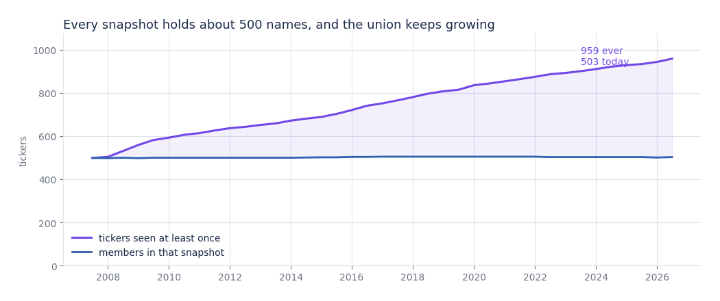
959 tickers were index members at some point in the window, against roughly 500 at any given moment. Those extra 459 are what a naive pull silently drops.
Every ticker that was ever a member gets downloaded, including the ones that no longer trade. Each stock then contributes rows only on the dates it was genuinely a member, enforced with a boolean mask. This matters twice over, because the target is a cross sectional comparison: a non member sitting in the panel would also distort the median every other stock is measured against.
Slow cell, and cached to disk afterwards
PRICES = Path("precos.parquet")

if PRICES.exists():
    px = pd.read_parquet(PRICES).astype("float32")
else:
    parts = []
    for i in range(0, len(universe), 120):
        d = yf.download(universe[i:i + 120], start=START, end=END,
                        auto_adjust=True, progress=False)
        if isinstance(d.columns, pd.MultiIndex):
            d = d["Close"]
        parts.append(d)
    px = pd.concat(parts, axis=1).sort_index()
    px = px.loc[:, ~px.columns.duplicated()].dropna(axis=1, how="all")
    px.to_parquet(PRICES)

# a cache written by a wider run would silently change the number of windows
px = px.loc[(px.index >= START) & (px.index <= END)]

marks = sorted(snapshots)
mask = pd.DataFrame(False, index=px.index, columns=px.columns)
for i, d0 in enumerate(marks):
    d1 = marks[i + 1] if i + 1 < len(marks) else "2100-01-01"
    mask.loc[(px.index >= d0) & (px.index < d1),
             [t for t in snapshots[d0] if t in mask.columns]] = True

print(f"{px.shape[1]} of {len(universe)} tickers with data")
print(f"median members on a day: {int(mask.sum(axis=1).median())}")
# 640 of 959 tickers with data
# median members on a day: 342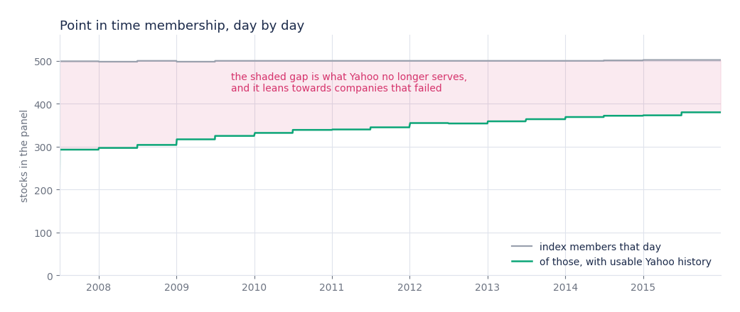
640 of the 959 have usable history, which is 67%. Yahoo no longer serves prices for many long delisted names, and the missing ones skew towards companies that failed, which is exactly the group whose absence causes the bias. Read this as a large improvement rather than a complete fix.
Asking "will the market go up" hands a model an upward drift it can free ride on. Krauss asks something relative instead: will this stock beat the median of its peers tomorrow. Half the universe beats the median every day by construction, so the base rate sits at 0.50 and no dumb rule is worth beating. Measured on the first window it comes out at 0.5005.
Features are 31 cumulative returns and nothing else. Every lookback from 1 to 20 trading days, then 40, 60 and so on to 240. No RSI, no moving average distance, no volatility. Short lookbacks carry reversal, long ones carry momentum, and the models are left to work out which applies where.
Each column is then standardised across the cross section of its own day, which is what makes different regimes comparable. A 2% return in October 2008 and a 2% return in a quiet stretch of 2014 mean different things, while "1.3 standard deviations above today's average" means the same thing in both.
frames = {}
for m in PERIODS:
    r  = (px / px.shift(m) - 1).where(mask)          # cumulative return over m days
    mu = r.mean(axis=1)                              # today's cross sectional mean
    sd = r.std(axis=1).replace(0, np.nan)
    frames[f"r_{m}"] = r.sub(mu, axis=0).div(sd, axis=0).astype("float32")

r1 = (px.shift(-1) / px - 1).where(mask)             # tomorrow's return
y_all = (r1.rank(axis=1, pct=True) > 0.5).astype("float32").where(r1.notna())

def stack(window):
    """Long format for one slice of dates: one row per stock per day."""
    X = pd.concat({n: f.loc[window].stack() for n, f in frames.items()}, axis=1)
    y = y_all.loc[window].stack().reindex(X.index)
    ok = y.notna() & X.notna().all(axis=1)
    return X[ok].astype("float32"), y[ok].astype("int8")

first = px.index[max(PERIODS):max(PERIODS) + TRAIN]
X0, y0 = stack(first)
print(f"{len(X0):,} rows x {X0.shape[1]} features")
print(f"window {first[0].date()} to {first[-1].date()}, target mean {y0.mean():.4f}")
# 216,952 rows x 31 features
# window 2007-12-14 to 2010-12-06, target mean 0.5005
Fitting one shallow tree on that first window, before any of the machinery below, already shows the whole problem in one picture.
One tree, three levels deep, drawn the way scikit-learn draws it
from sklearn.tree import DecisionTreeClassifier, plot_tree

shallow = DecisionTreeClassifier(max_depth=3, min_samples_leaf=500, random_state=0)
shallow.fit(X0, y0)

fig, ax = plt.subplots(figsize=(13.5, 5.4))
plot_tree(shallow, feature_names=list(X0.columns), class_names=["below", "above"],
          filled=False, impurity=False, proportion=True, rounded=False, fontsize=8, ax=ax)
plt.show()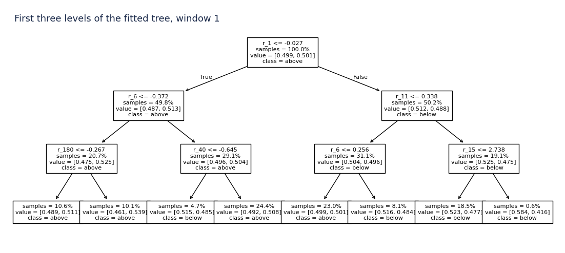
r_1, yesterday's return, at −0.027 standard
deviations: short term reversal is the first thing the tree finds. Read the leaves and the
whole page falls into place. Most hold 0.49 to 0.52, which is why AUC lands near 0.51, and
the one useful leaf holds 0.584 on 0.6% of the rows. A strategy that trades only the
extremes is built to hold exactly that leaf.Building the panel one window at a time rather than all at once is deliberate. Stacking twenty years of 640 stocks against 31 columns in memory is a few gigabytes; stacking 750 days of it is a few hundred megabytes, and each window is discarded before the next is built.
Everything from here to Step 6 rebuilds one specific paper: Deep neural networks, gradient-boosted trees, random forests: Statistical arbitrage on the S&P 500, by Krauss, Do and Huck, published in the European Journal of Operational Research in 2017. Only the three tree based models are reproduced here, since neural networks belong in a separate post.
Reproducing a paper is a better exercise than inventing a strategy, because the answer is written down in advance. If the numbers come out far from theirs, the pipeline is wrong until proven otherwise, which is a much healthier default than admiring your own backtest.
Every trading day, rank all index members by the probability that each one beats the cross-sectional median return tomorrow. Buy the top k, sell the bottom k, hold one day, repeat. Deliberately throw away the middle of the ranking, where the model has no conviction.
Their features are unusually plain: 31 cumulative returns and nothing else. Daily out to twenty days, then twenty day steps to 240, which is one trading year. No moving averages, no RSI, no volatility, no fundamentals.
Their reported results, over December 1992 to October 2015 with k = 10:
| Model | Return/day | t-stat | After costs | t-stat | Sharpe, net |
|---|---|---|---|---|---|
| Random forest | 0.43% | 14.93 | 0.23% | 7.91 | 1.90 |
| Gradient boosted trees | 0.37% | 12.68 | 0.17% | 5.90 | 1.23 |
| Deep neural network | 0.33% | 8.62 | 0.13% | 3.38 | 0.55 |
| Market | 0.04% | 2.83 | 0.35 |
Worth noting they charged 0.05% per share per half turn and the result still survived at t = 7.91. Worth noting too that a gross Sharpe of 5.12 is extraordinary for a published equity strategy, and their own net figure of 1.90 is the more believable of the two.
One fixed train and test split would be wrong here, because a model fitted in 2010 and asked about 2015 has never seen the regime it is trading. Instead the window slides: train on 750 days, trade the next 250, move forward 250 days and refit from scratch.
Features, target and the sliding window
PERIODS = list(range(1, 21)) + list(range(40, 241, 20))    # 31 features
TRAIN, TRADE = 750, 250

frames = {}
for m in PERIODS:
    r = (px / px.shift(m) - 1).where(mask)                 # only past prices
    mu, sd = r.mean(axis=1), r.std(axis=1).replace(0, np.nan)
    frames[f"r_{m}"] = r.sub(mu, axis=0).div(sd, axis=0)   # standardised across the day

r1 = (px.shift(-1) / px - 1).where(mask)                   # TOMORROW's return
y  = (r1.rank(axis=1, pct=True) > 0.5).astype("float32").where(r1.notna())

windows = range(max(PERIODS), len(days) - TRAIN - TRADE, TRADE)
for i in windows:
    train_days = days[i : i + TRAIN]
    trade_days = days[i + TRAIN : i + TRAIN + TRADE]
    model.fit(*stack(train_days))                          # refit from scratch each window
    p = model.predict_proba(stack(trade_days)[0])[:, 1]
    # long the top k probabilities of each day, short the bottom k
    for d, group in p.groupby(level=0):
        order = group.sort_values(ascending=False)
        ret = r1.loc[d, order.index[:k]].mean() - r1.loc[d, order.index[-k:]].mean()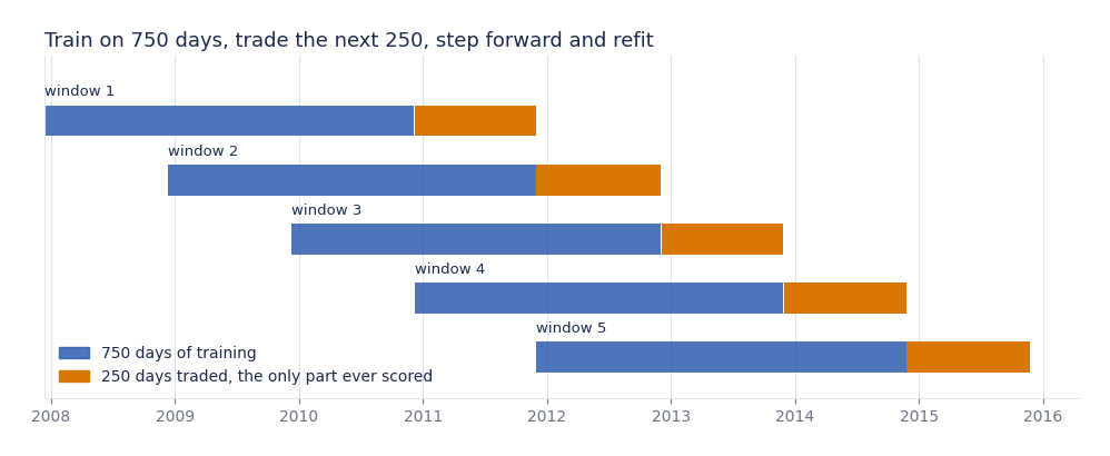
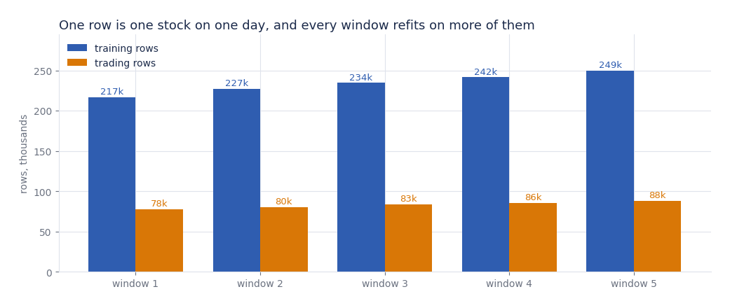
| Window | Trains on | Trades, out of sample | Training rows | Trading rows | Target mean |
|---|---|---|---|---|---|
| 1 | 2007-12-14 to 2010-12-06 | 2010-12-07 to 2011-12-01 | 216,952 | 77,821 | 0.5007 |
| 2 | 2008-12-11 to 2011-12-01 | 2011-12-02 to 2012-11-30 | 227,092 | 80,244 | 0.5012 |
| 3 | 2009-12-09 to 2012-11-30 | 2012-12-03 to 2013-11-27 | 234,473 | 83,488 | 0.5002 |
| 4 | 2010-12-07 to 2013-11-27 | 2013-11-29 to 2014-11-25 | 241,553 | 85,730 | 0.5003 |
| 5 | 2011-12-02 to 2014-11-25 | 2014-11-26 to 2015-11-23 | 249,462 | 88,044 | 0.5006 |
Same five rows carry the results further down, once the models have run. Target mean sits on 0.500 in every trading block, which is the balance being enforced rather than assumed: any model that cannot clear 0.50 has learned nothing at all.
One deviation from the paper is worth declaring. Krauss standardises each feature over its own history; Step 4 standardises across the cross-section of the day instead, which suits a target that is itself cross-sectional and keeps every column on one scale within a day.
Five windows, each trained on 750 days and traded on the 250 that follow. Every number below comes from the trading columns only, so no model is ever scored on data it was fitted on.
| Window | Trains on | Trades | Tree | Forest | Boosting |
|---|---|---|---|---|---|
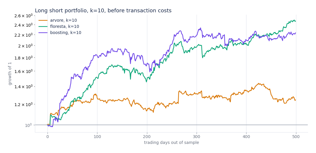
| 1 | 2007-12-14 to 2010-12-06 | 2010-12-07 to 2011-12-01 | +0.081% | +0.265% | +0.295% |
| 2 | 2008-12-11 to 2011-12-01 | 2011-12-02 to 2012-11-30 | +0.019% | +0.115% | +0.048% |
| 3 | 2009-12-09 to 2012-11-30 | 2012-12-03 to 2013-11-27 | +0.046% | +0.124% | +0.002% |
| 4 | 2010-12-07 to 2013-11-27 | 2013-11-29 to 2014-11-25 | +0.120% | +0.116% | +0.081% |
| 5 | 2011-12-02 to 2014-11-25 | 2014-11-26 to 2015-11-23 | +0.010% | +0.182% | +0.188% |
Every cell is positive. That consistency matters more than the average, because a strategy carried by one lucky year looks identical to a real one once you take the mean.
| Model | Return/day | Annualised | t-stat | p | Windows positive |
|---|---|---|---|---|---|
| Decision tree | 0.055% | 14.9% | 2.02 | 0.044 | 5 of 5 |
| Random forest | 0.160% | 49.7% | 4.80 | <0.0001 | 5 of 5 |
| XGBoost | 0.123% | 36.3% | 3.36 | 0.0008 | 5 of 5 |
Roughly 37% of the paper's headline figure, in the same direction, with the same ordering of models. Close enough to call the pipeline sound, and short enough to be worth explaining: our overlap with their sample is 2010 to 2015, the tail end where they report profits already declining, and our universe is smaller than theirs.
AUC asks a single question: take one stock that did beat the median and one that did not, and how often does the model give the winner the higher probability? A score of 0.50 means it is guessing. A score of 1.00 means it is never wrong.
Accuracy answers a different question, how many calls land on the right side of a threshold, and it can be flattered by an unbalanced target. Here the target is balanced 50/50 by construction, so AUC is the cleaner measure of whether the ranking itself is any good.
Curves in sample and out of sample
from sklearn.metrics import roc_curve, roc_auc_score

model.fit(Xtr, ytr)
p_train, p_test = model.predict_proba(Xtr)[:, 1], model.predict_proba(Xte)[:, 1]

for y_, p_, label in [(ytr, p_train, "train"), (yte, p_test, "test")]:
    fpr, tpr, _ = roc_curve(y_, p_)
    plt.plot(fpr, tpr, label=f"{label}  {roc_auc_score(y_, p_):.3f}")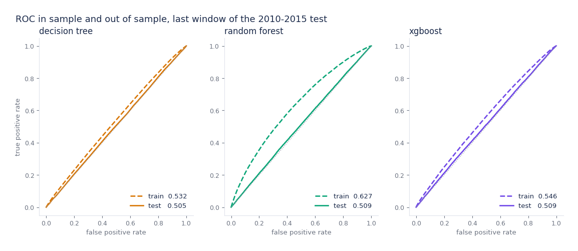
| Model | Train | Test | Gap |
|---|---|---|---|
| Decision tree | 0.5366 | 0.5048 | 0.0318 |
| Random forest | 0.6315 | 0.5071 | 0.1244 |
| XGBoost | 0.5485 | 0.5076 | 0.0409 |
Now hold those two facts together. Out of sample the models score 0.51, which is a hair above guessing. Over the same period they earned 0.16% a day. Both are true, and reconciling them is the most useful thing on this page.
AUC scores the whole ranking, most of which is noise the strategy never touches. The strategy only trades the ten names at each end, where conviction is highest. A model can be almost useless on average and still be right slightly more often at the extremes, and one day of that, compounded 250 times a year across 20 positions, is where the return comes from.
Read in reverse, this is also why a high AUC on a page like this would be a warning sign rather than a triumph.
Three biases would each be enough to invent this result. Each one is checked by running a test rather than by asserting it, and the script prints all four.
Features use closing prices up to today. The target uses the return from today's close to tomorrow's. If those ever crossed, the result would be meaningless.
d = days[1200]
today    = px.loc[d, s] / px.loc[days[1199], s] - 1
tomorrow = px.loc[days[1201], s] / px.loc[d, s] - 1
assert abs(r1.loc[d, s] - tomorrow) < 1e-9        # target matches TOMORROW, not today

# on 2011-10-06 for ticker A:
#   today    +0.04421
#   tomorrow -0.06470
# stored -0.06470 correctIndex membership is rebuilt from the Wikipedia revision history, as in Step 2, so a company contributes rows only while it was genuinely a member.
# snapshot in force on 2011-10-06 lists 500 names
#   345 of our tickers are active in the panel that day
#   295 exist in the price file but are correctly excluded
#
# 959 tickers were index members at some point, 503 are members today
# 141 of the departed are still in the panel, e.g. AA, AAL, AAP, ACT, ADT, AIV, ALK, AMG
Those 141 names are the point. A long short strategy earns roughly a third of its return on the short leg, and companies that fell out of the index are exactly the population a short book wants. Drop them and the backtest improves for a reason that has nothing to do with the model.
Nothing above changes except the dates. Same features, same window lengths, same models, same universe, extended to fifteen consecutive windows ending November 2025. Grouping them in blocks of five shows where the edge went.
| Traded | Tree | Forest | Boosting |
|---|---|---|---|
| 2010 to 2015 | +0.055% | +0.160% | +0.123% |
| 2015 to 2020 | −0.019% | +0.098% | +0.081% |
| 2020 to 2025 | +0.028% | +0.031% | −0.012% |
Forest returns fall by roughly half, then by half again. Boosting goes negative in the last block. Pooled across all fifteen windows the forest still reads 0.097% a day at t = 3.97, significant on paper, but that number is carried almost entirely by the first third of the sample and would be a poor guide to what the next window pays.
Two readings fit the data equally well and this test cannot separate them. Either the anomaly was arbitraged away as these methods became standard, which is the direction the paper itself documents after 2001, or it survives and needs more than 31 momentum features to reach. Either way the honest summary is that a published edge reproduced on the period it was published for, and did not persist at that size afterwards.
Reproducing the fifteen window sweep
# the five window replication of the paper period
python krauss.py --desde 2007-01-01 --ate 2015-12-31

# every window through to 2025, roughly 40 minutes on a laptop
python krauss.pyPCA is not a predictor at all, it is unsupervised compression, and it is where machine learning starts genuinely paying for itself in finance.
Ten Treasury maturities move together almost all of the time, so treating them as ten independent risks is wasteful and unstable. PCA finds the eigenvectors of their covariance matrix, rotating the ten correlated series into uncorrelated components ordered by how much variance each one carries:
Σ vk = λk vk
so that Δyt ≈ Σk=1..3 ck,t vk
Run it on daily changes in yield rather than levels. Levels are non-stationary and the first component would simply track the drift of the whole rate era.
Three components from ten maturities
from sklearn.decomposition import PCA

tenors = ["DGS3MO","DGS6MO","DGS1","DGS2","DGS3","DGS5","DGS7","DGS10","DGS20","DGS30"]
curve  = fred(tenors).dropna()

p = PCA(n_components=5).fit(curve.diff().dropna())      # CHANGES, not levels
print(p.explained_variance_ratio_)
# [0.7827  0.1351  0.0386  0.0190  0.0079]

level, slope, curvature = p.components_[:3]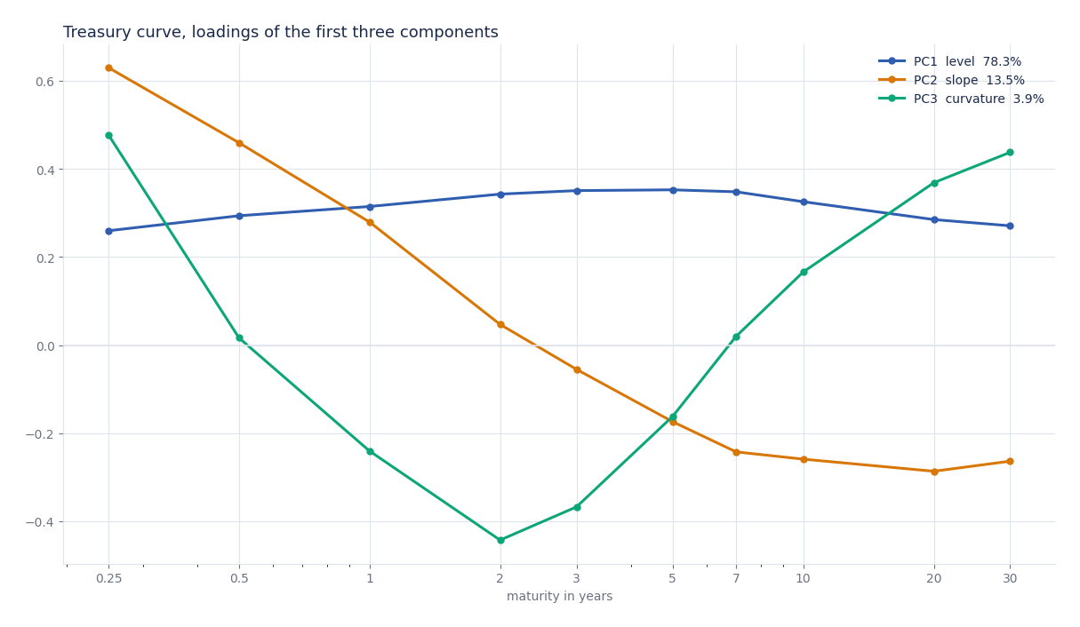
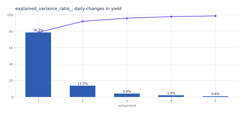
| Component | Shape | Variance explained | Cumulative |
|---|---|---|---|
| PC1 | Level | 78.27% | 78.27% |
| PC2 | Slope | 13.51% | 91.78% |
| PC3 | Curvature | 3.86% | 95.64% |
| PC4 | 1.90% | 97.54% | |
| PC5 | 0.79% | 98.33% |
PCA answers a narrower question than the sections above, and answers it cleanly. Stable, interpretable, and exactly what a fixed income desk trades: hedge three risks rather than ten that move together, and the components hold their shape well enough across regimes that the hedge does not need refitting every month. The same machinery compresses a factor covariance matrix before it reaches a portfolio optimiser.
One caveat worth stating. Requiring all ten maturities to be present drops the window where the 30 year bond was discontinued, between February 2002 and February 2006. The sample is long but it has a hole in it.
Linear regression carrying a penalty on the size of its own coefficients:
minβ ‖y − Xβ‖² + λ‖β‖1
The L1 norm is what makes this different from ridge regression. Its constraint region has corners on the axes, and the optimum tends to land on one, which drives coefficients to exactly zero rather than merely shrinking them. In the orthogonal case the solution is literally a soft threshold:
β̂j = sign(zj) · (|zj| − λ)+
So the model selects its variables while it fits them, in one pass, and λ sets how short the surviving list runs. That is exactly what equity factor research needs. With a hundred candidate signals and twenty years of monthly data, ordinary least squares fits noise and reports it as skill. Here the target is the forward 21 day SPY return, and the candidates are 21 day momentum and realised volatility for 22 sector and asset class ETFs, plus six macro series from FRED.
Lasso with time series cross validation
from sklearn.linear_model import LassoCV
from sklearn.preprocessing import StandardScaler
from sklearn.model_selection import TimeSeriesSplit

scaler = StandardScaler().fit(panel[:cut])          # fit on TRAIN only, never the full sample

cv = LassoCV(
    cv=TimeSeriesSplit(5),                          # temporal folds, never shuffled
    n_alphas=120,
    max_iter=20000,
    random_state=0,
).fit(scaler.transform(panel[:cut]), fwd[:cut])

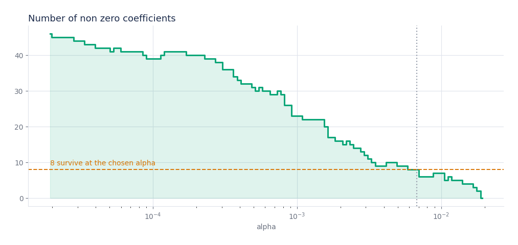
alive = [c for c, b in zip(panel.columns, cv.coef_) if abs(b) > 1e-10]
print(len(alive), "of", panel.shape[1])
# 8 of 50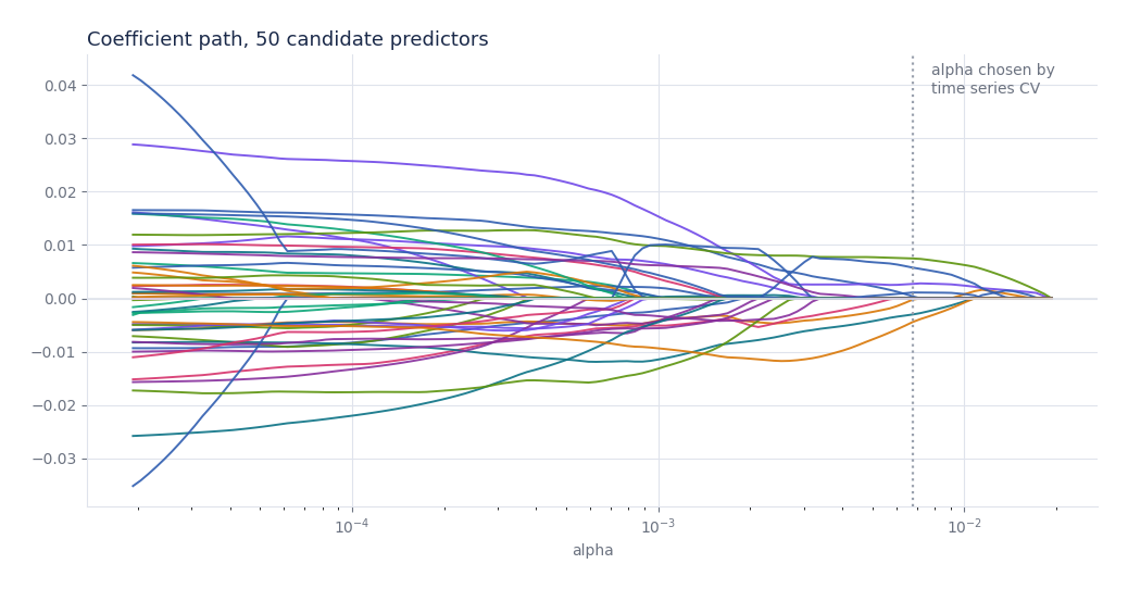
| Measure | Value |
|---|---|
| Candidate predictors | 50 |
| Non zero coefficients | 8 |
| Out of sample R² | 0.0908 |
| R² of predicting the training mean | −0.0080 |
An out of sample R² of 0.09 is small in absolute terms and it is the only positive result among the five predictive attempts. It is also the shape of result you should expect: a monthly horizon is far more forecastable than a weekly direction, and the survivors are the sensible ones. High yield credit spreads and the dollar index came through, alongside realised volatility on gold, small caps, oil and real estate, and momentum on developed international and energy. Credit and the dollar carrying information about forward equity returns is an old idea, and the Lasso found it without being told.
Treat it as a research filter rather than a strategy. There is no transaction cost here, no slippage, and a single asset, which are three of the ways a result like this usually disappears.
Everything on this page as one runnable Jupyter notebook. Same cells, same order, same numbers. Join the newsletter (free) and the download is yours.
Write your name and a valid email to unlock the download.
machine_learning_finance.ipynb
Enter your name & email above to unlock
Free. One short email when there's something new. No spam, unsubscribe in one click.
Everything above is reproducible from the notebook and no paid data. What follows is the list of things that are still wrong with it, because a results page without one is asking to be believed rather than checked.
auto_adjust=True applies
today's split and dividend factors across the whole history, so a 2010 price reflects
adjustments decided later. Standard practice, and harmless for ranking, but not strictly
point in time.
None of this makes the exercise pointless. It makes it a worked example, which is what it is for: the pipeline, the honest evaluation and the order of magnitude to expect. For work that has money behind it, start from the literature instead, and five machine learning papers that reshaped quant finance is a reasonable first stop.
| Model | Task | Result | Benchmark | Verdict |
|---|---|---|---|---|
| Decision tree | Beat tomorrow's median | 0.055%/day, t = 2.02 | 0.43%/day in the paper | Same sign, thin |
| Random forest | Beat tomorrow's median | 0.160%/day, t = 4.80 | 0.43%/day in the paper | Reproduces at 37% |
| XGBoost | Beat tomorrow's median | 0.123%/day, t = 3.36 | 0.37%/day in the paper | Reproduces at 33% |
| PCA | Curve structure | 95.64% in 3 components | 10 correlated maturities | Strong, and stable |
| Lasso | 21 day return | R² 0.0908 | −0.0080 for the mean | Small but real |
Three tree based classifiers rank stocks barely better than chance, AUC 0.51 against 0.50, and still earn a real spread because a long short book only ever touches the two ends of that ranking. Both facts are true at once, and holding them together is what separates a usable signal from a broken one.
Scale is the thing to carry away. A published, peer reviewed, widely cited strategy delivers roughly a sixth of a percent a day before costs on the period it was written about, and roughly a thirtieth of that by 2025. Any backtest reporting far more, on free daily data and price features alone, is worth reading twice.
PCA and Lasso are doing different work. PCA was not asked to forecast anything, only to describe a covariance structure that genuinely exists, and it recovered level, slope and curvature without being told they were there. Lasso was given a longer horizon and a wide candidate set, so selection became the useful output.
A good model is not the one with the highest score. It is the one that keeps scoring out of sample, on a temporal split, on a universe that includes the companies that failed, measured against the dumb alternative. Drop any one of those and every backtest starts to look brilliant.
Neural networks are deliberately absent, which is why only three of the paper's four models appear here. Krauss tested a deep feedforward network as well, and among single models the random forest came out ahead of it. Deep learning on tabular financial data carries its own failure modes and deserves separate treatment rather than a sixth section here.