Heston Volatility Surface in Python

1. What Heston is, in two SDEs

Black-Scholes assumes volatility is a constant. The market politely disagrees. Implied vol moves around every minute, the smile is asymmetric, and short-dated options price in a steeper skew than long-dated ones. None of that fits a single number.

The Heston model fixes the gap by letting variance itself be a stochastic process. The stock follows the usual lognormal dynamics, but the variance $v_t$ now has its own SDE with mean reversion and noise:

$$dS_t \;=\; r\,S_t\,dt \;+\; \sqrt{v_t}\,S_t\,dW_t^{(1)}$$

$$dv_t \;=\; \kappa(\theta - v_t)\,dt \;+\; \xi\,\sqrt{v_t}\,dW_t^{(2)}$$

$$\mathrm{corr}\,\!\bigl(dW^{(1)},\, dW^{(2)}\bigr) \;=\; \rho$$

That single change buys you four things Black-Scholes can't produce:

Skew. $\rho$ controls how asymmetric the smile is. $\rho < 0$ (the equity leverage effect) tilts the smile to the left: OTM puts trade richer than OTM calls.
Curvature. $\xi$ is the vol of vol. Higher $\xi$ widens the wings — fatter tails on the implied distribution, more bowed smile.
Term structure. $\kappa$ and $\theta$ describe how fast variance reverts to its long-run level, so the smile shape depends on $T$.
Stochastic vol regimes. $v_t$ itself evolves over time. Today's surface depends on today's $v_t$, not on a static input.

Five parameters, five things to think about: $\rho$, $\xi$, $\kappa$, $\theta$, $v_0$. The rest of this notebook is a 1D walk through each one, then the 3D surface, then a side-by-side of how the surface morphs when $v_0$ shifts from a low-vol to a high-vol regime.

2. Setup

Heston option prices aren't closed-form like Black-Scholes. The standard route is the characteristic function $\varphi(u)$ of $\log S_T$ — a complex-valued function we can integrate numerically (via Lewis-style Fourier inversion) to get the call price. We'll then invert that price into an implied vol with Brent's root finder against the Black-Scholes formula.

Three libraries: numpy for arrays, scipy for the integral and the root finder, matplotlib for the plots.

pip install numpy scipy matplotlib

Imports + the characteristic function + the Heston call pricer + Black-Scholes inversion:

import numpy as np
from scipy.integrate import quad
from scipy.optimize import brentq
from scipy.stats import norm

# Defaults we will reuse below (equity-vol regime).
S0, R, Q       = 100.0, 0.03, 0.00
V0, KAPPA      = 0.019, 2.5
THETA, XI, RHO = 0.07,  0.75, -0.72

def heston_char(u, T, S0, r, q, v0, kappa, theta, xi, rho):
    """Albrecher 'little trap' form of the Heston characteristic function."""
    u    = np.asarray(u, dtype=complex)
    xi_h = kappa - rho * xi * 1j * u
    d    = np.sqrt(xi_h**2 + xi**2 * (u * 1j + u**2))
    g2   = (xi_h - d) / (xi_h + d)
    C    = (kappa * theta / xi**2) * (
        (xi_h - d) * T - 2.0 * np.log((1 - g2 * np.exp(-d * T)) / (1 - g2))
    )
    D    = ((xi_h - d) / xi**2) * (1 - np.exp(-d * T)) / (1 - g2 * np.exp(-d * T))
    return np.exp(C + D * v0 + 1j * u * (np.log(S0) + (r - q) * T))

def heston_call(K, T, *, S0=S0, r=R, q=Q, v0=V0,
                kappa=KAPPA, theta=THETA, xi=XI, rho=RHO):
    """Heston European call via Fourier-style numerical integration."""
    args = dict(S0=S0, r=r, q=q, v0=v0, kappa=kappa, theta=theta, xi=xi, rho=rho)
    def p1(u):
        return np.real(np.exp(-1j*u*np.log(K)) * heston_char(u - 1j, T, **args)
                       / (1j*u * heston_char(-1j, T, **args)))
    def p2(u):
        return np.real(np.exp(-1j*u*np.log(K)) * heston_char(u, T, **args) / (1j*u))
    P1 = 0.5 + (1.0/np.pi) * quad(p1, 1e-8, 100, limit=200)[0]
    P2 = 0.5 + (1.0/np.pi) * quad(p2, 1e-8, 100, limit=200)[0]
    return S0 * np.exp(-q*T) * P1 - K * np.exp(-r*T) * P2

def bs_call(K, T, sigma, S0=S0, r=R, q=Q):
    """Black-Scholes call (used as the inversion target)."""
    d1 = (np.log(S0/K) + (r - q + 0.5*sigma**2)*T) / (sigma*np.sqrt(T))
    d2 = d1 - sigma*np.sqrt(T)
    return S0*np.exp(-q*T)*norm.cdf(d1) - K*np.exp(-r*T)*norm.cdf(d2)

def implied_vol(price, K, T, S0=S0, r=R, q=Q):
    """Invert a call price to BS implied vol using Brent's method."""
    intrinsic = max(S0*np.exp(-q*T) - K*np.exp(-r*T), 0.0)
    if price <= intrinsic + 1e-8:
        return np.nan
    try:
        return brentq(lambda s: bs_call(K, T, s, S0, r, q) - price, 1e-4, 5.0, xtol=1e-6)
    except (ValueError, RuntimeError):
        return np.nan

3. Reading the parameters in practice

Before slicing the surface, a sanity check: what do these five parameters actually look like for real assets? The Heston model is calibrated to listed option prices, and the calibrated values differ wildly across asset classes. Equity indices, single names, bonds, gold, and crypto all live in very different corners of the parameter space.

The table below shows order-of-magnitude calibrated Heston parameters across five representative underlyings. Take it as a "feel for the numbers" rather than a quotation — actual calibrations depend on the date, the option chain you fit, and the moneyness window.

Underlying	$\kappa$ (mean rev.)	$\theta$ (long-run var)	$\xi$ (vol of vol)	$\rho$ (skew)	$v_0$ (today)	Short-dated ATM vol
SPY (S&P 500)	2.5	0.040	0.75	−0.75	0.020	~14%
AAPL (single name)	1.5	0.070	1.20	−0.55	0.045	~21%
TLT (20+ yr Treasury)	3.0	0.018	0.45	+0.05	0.015	~12%
GLD (gold ETF)	2.0	0.025	0.55	−0.10	0.022	~15%
BTC (crypto, weekly)	0.8	0.500	2.50	−0.30	0.400	~63%

Four patterns to read off the table:

Equity indices carry the strongest negative $\rho$. SPY sits at $\rho \approx -0.75$. This is the leverage effect: when the index falls, vol spikes. It is the structural reason for the deep put-side skew in S&P options. Single names show the same sign but weaker magnitude because idiosyncratic noise dilutes the index-level correlation.
Single names have higher vol of vol than the index. AAPL sits at $\xi \approx 1.20$ vs SPY at $0.75$. Diversification dampens index variance fluctuations; a single stock can double its vol on an earnings miss, so $\xi$ has to be larger to fit its option chain.
Bond options have $\rho \approx 0$ or slightly positive. The leverage effect doesn't apply: the relationship between bond price moves and bond vol isn't asymmetric the same way as equities. TLT options price in roughly symmetric smiles, with $\xi$ also lower because rates vol is structurally less explosive than equity vol.
Crypto lives in a different universe. $\theta$ of $0.50$ corresponds to a long-run vol of $\sqrt{0.50} \approx 71\%$. $\xi = 2.5$ is more than 3x SPY. The Heston model still fits crypto, but the calibrated parameters look almost unrecognisable next to a listed equity option.

One useful exercise once you have the code below working: plug in any row from this table and re-run the 1D slices. The smile under SPY parameters will look very different from the same smile under TLT or BTC. The rest of the notebook uses the SPY-style equity-vol regime as the default (matching the values printed in section 2), but every plotting cell takes keyword overrides so you can swap any subset of parameters in one line.

3.1 What each parameter actually controls on the surface

Before the 1D plots, a one-line summary of what each parameter does to the surface — so when you see the slices below, you already know which knob is being turned.

$\rho$ — left-right tilt of the smile. Negative tilts the smile down on the put side. Set the skew direction.
$\xi$ — how bowed the smile is. Higher $\xi$ = wider wings.
$\kappa$ — speed at which the term structure flattens. Higher $\kappa$ = faster convergence to $\sqrt{\theta}$.
$\theta$ — the long-run vol level the surface mean-reverts to. Sets the "floor" at long $T$.
$v_0$ — today's variance state. Shifts the whole surface up or down. Doesn't change skew or curvature.

Now to the 1D slices. Each section below isolates one parameter, holds the others at the defaults, and walks the value across a sensible range so you can see its effect cleanly.

4. Smile vs Strike — effect of $\rho$ (the skew control)

Fix everything else and only vary $\rho$. The smile tilts. $\rho < 0$ means a negative shock to the asset is correlated with a positive shock to its variance — the equity-vol "leverage effect". OTM puts price in higher vol than OTM calls, and the smile becomes a downward-sloping line of skew. As $\rho$ moves toward zero the smile becomes symmetric, and a positive $\rho$ flips the asymmetry the other way.

import matplotlib.pyplot as plt

T_fixed = 0.30
strikes = np.linspace(80, 120, 35)

plt.figure(figsize=(9, 5.2))
for rho_val in [-0.9, -0.5, 0.0, 0.3]:
    ivs = [implied_vol(heston_call(K, T_fixed, rho=rho_val), K, T_fixed) for K in strikes]
    plt.plot(strikes, np.array(ivs)*100, lw=2.4, label=f"rho = {rho_val:+.1f}")
plt.axvline(S0, color="gray", ls="--", lw=0.8, label=f"Spot K = {S0:.0f}")
plt.title(f"Heston smile vs Strike — effect of rho   (T = {T_fixed}, v_0 = {V0}, xi = {XI})")
plt.xlabel("Strike K"); plt.ylabel("Implied Vol (%)")
plt.legend(); plt.grid(True); plt.tight_layout(); plt.show()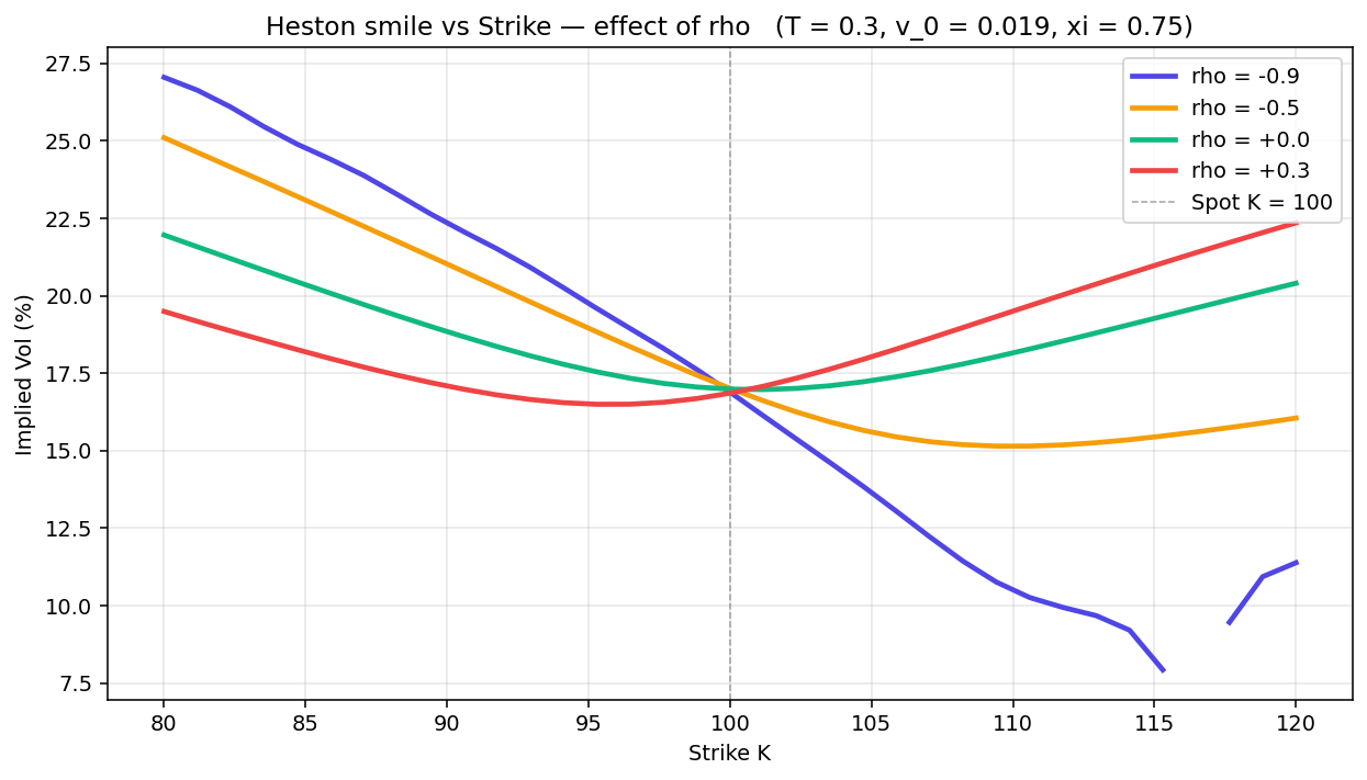

Heston smile vs strike, four different rho values, showing skew direction flip

Pure rotation around the ATM strike. Strong negative $\rho$ (blue, $\rho = -0.9$) produces a deep left-skew — the equity vol leverage effect at full strength. Positive $\rho$ (red, $\rho = +0.3$) does the opposite. The deep-OTM noise on the $\rho = -0.9$ curve is the BS inversion hitting near-intrinsic prices, not a model error.

5. Smile vs Strike — effect of $\xi$ (the vol of vol)

$\xi$ is the diffusion coefficient of the variance SDE. Intuitively: how violently variance kicks around. Higher $\xi$ means variance has a wider distribution at any future date, which fattens the tails of the implied $\log S_T$ distribution, which makes the smile more bowed. Low $\xi$ collapses the smile toward a flat Black-Scholes line.

plt.figure(figsize=(9, 5.2))
for xi_val in [0.2, 0.5, 1.0, 1.5]:
    ivs = [implied_vol(heston_call(K, T_fixed, xi=xi_val), K, T_fixed) for K in strikes]
    plt.plot(strikes, np.array(ivs)*100, lw=2.4, label=f"xi = {xi_val}")
plt.axvline(S0, color="gray", ls="--", lw=0.8, label=f"Spot K = {S0:.0f}")
plt.title(f"Heston smile vs Strike — effect of xi (vol of vol)   (T = {T_fixed}, rho = {RHO})")
plt.xlabel("Strike K"); plt.ylabel("Implied Vol (%)")
plt.legend(); plt.grid(True); plt.tight_layout(); plt.show()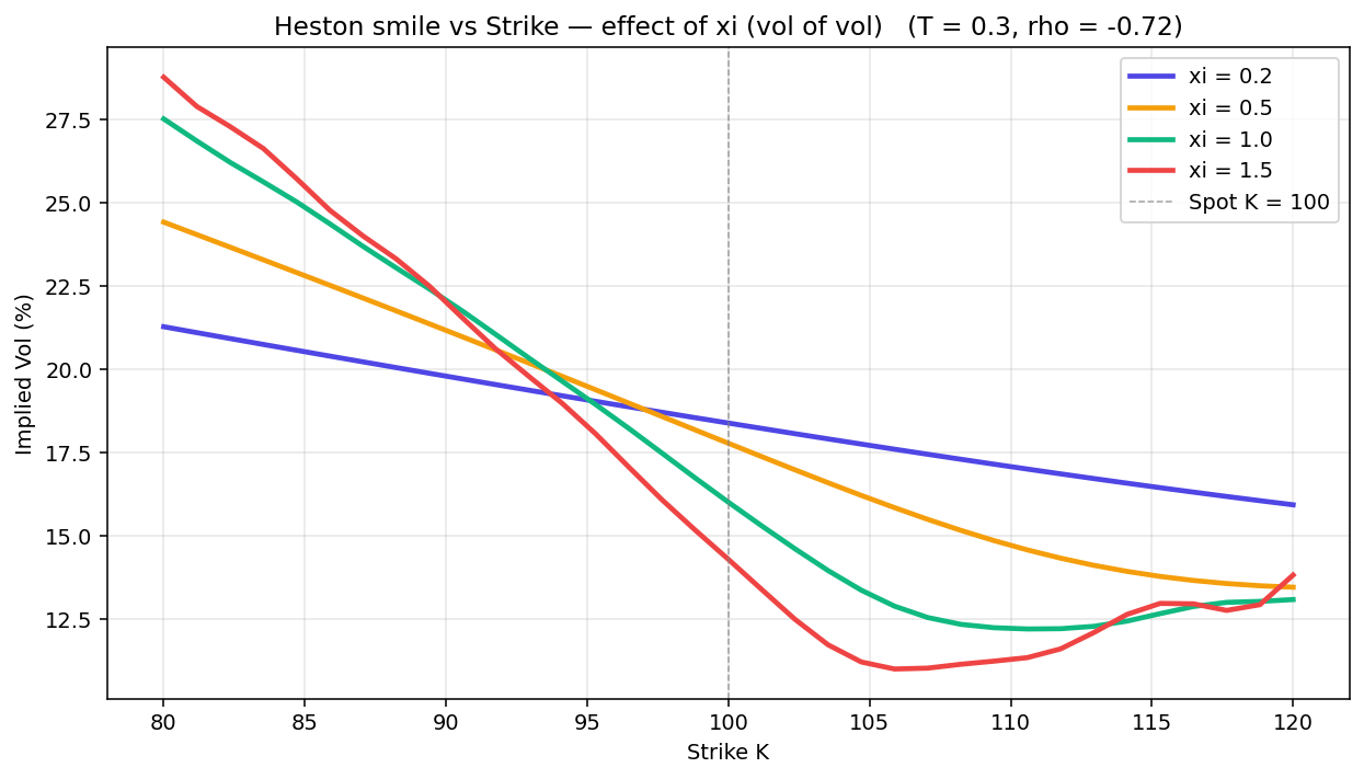

Heston smile vs strike for four xi values, showing curvature increase

Same midpoint, different wings. As $\xi$ grows the smile bows out — the wings demand a higher vol because variance can wander further by expiry. $\rho$ controls the left-right tilt, $\xi$ controls how much the wings lift up.

6. Smile across $T$ — the smile flattens as expiry grows

Keep all parameters at their defaults and walk the maturity instead. At short $T$, the variance hasn't had time to mean-revert, so the smile is steep and reflects all of $v_t$'s current asymmetry. At long $T$, the model averages over many possible variance paths and the smile flattens toward the long-run vol $\sqrt{\theta}$.

This is the single biggest reason BS doesn't fit real markets: the empirically observed flattening of the smile with $T$ is a stochastic-vol phenomenon, not a BS one.

plt.figure(figsize=(9, 5.2))
for T_val in [0.10, 0.50, 1.00]:
    ivs = [implied_vol(heston_call(K, T_val), K, T_val) for K in strikes]
    plt.plot(strikes, np.array(ivs)*100, lw=2.4, label=f"T = {T_val}")
plt.axvline(S0, color="gray", ls="--", lw=0.8, label=f"Spot K = {S0:.0f}")
plt.title("Heston smile flattens as T grows   (default Heston params)")
plt.xlabel("Strike K"); plt.ylabel("Implied Vol (%)")
plt.legend(); plt.grid(True); plt.tight_layout(); plt.show()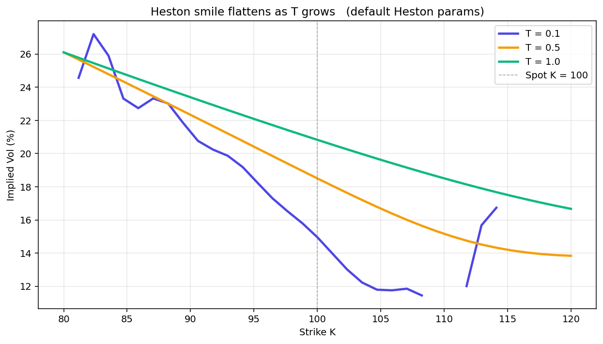

Three smiles at T = 0.10, 0.50, 1.00, demonstrating flattening

$T = 0.10$ gives the steepest, most asymmetric smile. By $T = 1.0$ the smile is noticeably flatter and the level is closer to $\sqrt{\theta}$. This is what "stochastic vol generalises Black-Scholes" actually looks like.

7. ATM term structure — effect of $\kappa$ (mean reversion speed)

Switch axes. Instead of plotting a smile at fixed $T$, plot the ATM implied vol as a function of $T$. The shape is now a "term structure" — short-dated vol on the left, long-dated vol on the right. $\kappa$ controls how fast it converges to its long-run level $\sqrt{\theta}$.

High $\kappa$ snaps the term structure flat quickly. Low $\kappa$ leaves a long transient where the surface still remembers the starting variance $v_0$.

def atm_term_structure(maturities, **overrides):
    ivs = np.full_like(maturities, np.nan, dtype=float)
    for i, T in enumerate(maturities):
        try:
            ivs[i] = implied_vol(heston_call(S0, T, **overrides), S0, T)
        except Exception:
            pass
    return ivs

Ts = np.linspace(0.1, 2.0, 24)
plt.figure(figsize=(9, 5.2))
for kappa_val in [0.5, 1.5, 3.0, 5.0]:
    ivs = atm_term_structure(Ts, kappa=kappa_val)
    plt.plot(Ts, ivs*100, lw=2.4, label=f"kappa = {kappa_val}")
plt.axhline(np.sqrt(THETA)*100, color="gray", ls="--",
            label=f"sqrt(theta) = {np.sqrt(THETA)*100:.1f}%")
plt.title(f"ATM term structure — effect of kappa  (v_0 = {V0}, theta = {THETA})")
plt.xlabel("Time to expiry T (years)"); plt.ylabel("ATM Implied Vol (%)")
plt.legend(); plt.grid(True); plt.tight_layout(); plt.show()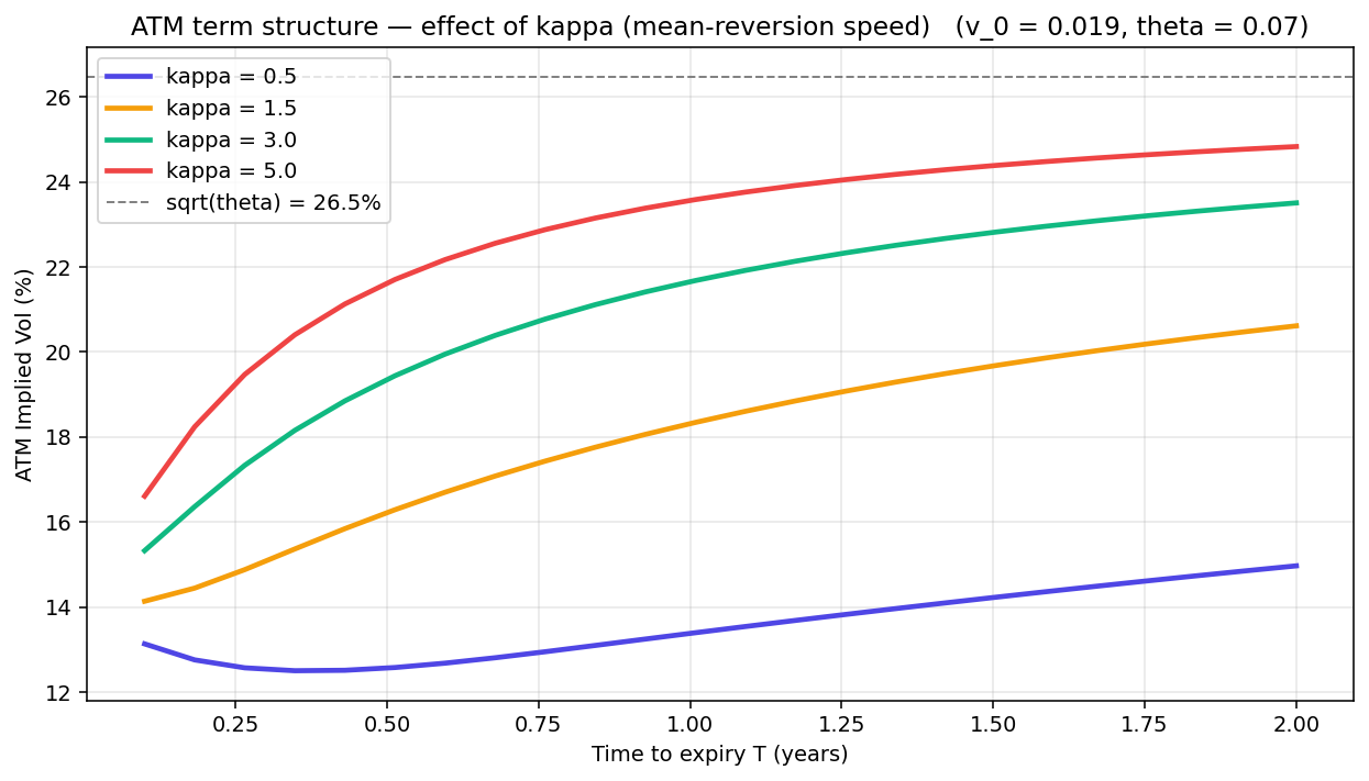

ATM term structure for four kappa values, all converging to sqrt(theta)

All four curves start from the same near-ATM short-dated vol and asymptote to $\sqrt{\theta}$. $\kappa = 5$ gets there fast; $\kappa = 0.5$ drags out the transition over the full 2-year window.

8. ATM term structure — effect of $v_0$ (the starting variance)

$v_0$ is "today's variance state". It's the only parameter on this page that's actually observed in the market (via short-dated ATM implied vol). Higher $v_0$ lifts the entire term structure; lower $v_0$ drops it. Both still mean-revert to $\sqrt{\theta}$ given enough time, just from a different starting point.

The reel at the top of this page animates $v_t$ along an SDE path. Each frame is a recomputed surface at the current $v_t$ — the breathing-up-and-down you see is exactly the four curves below shifting between regimes.

plt.figure(figsize=(9, 5.2))
for v0_val in [0.005, 0.02, 0.07, 0.15]:
    ivs = atm_term_structure(Ts, v0=v0_val)
    plt.plot(Ts, ivs*100, lw=2.4, label=f"v_0 = {v0_val}")
plt.axhline(np.sqrt(THETA)*100, color="gray", ls="--",
            label=f"sqrt(theta) = {np.sqrt(THETA)*100:.1f}%")
plt.title(f"ATM term structure — effect of v_0  (kappa = {KAPPA}, theta = {THETA})")
plt.xlabel("Time to expiry T (years)"); plt.ylabel("ATM Implied Vol (%)")
plt.legend(); plt.grid(True); plt.tight_layout(); plt.show()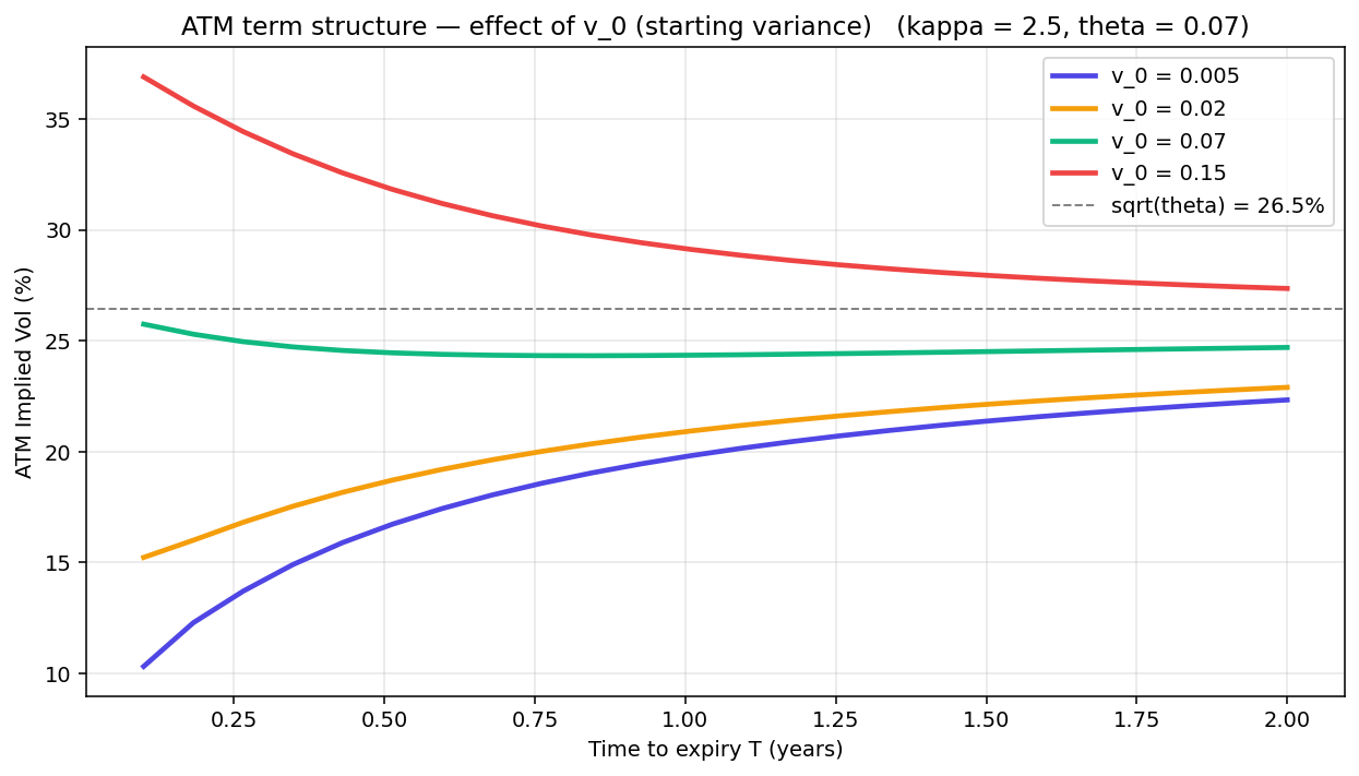

ATM term structure for four v_0 values, fan shape converging to sqrt(theta)

Fan-shape. Low starting variance ($v_0 = 0.005$, blue) climbs up to $\sqrt{\theta}$. High starting variance ($v_0 = 0.15$, red) decays down to the same level. The four curves cross only at the long end — that's the mean reversion of $v_t$ playing out.

9. Stacking it all: the 3D implied vol surface

With the 1D slices in hand, the 3D surface is just $IV(K, T)$ on a grid. Strike on one floor axis, expiry on the other, implied vol as the height. To see how the surface morphs with the state, the trick (same as the gamma page) is to compare two snapshots on the same z-axis: a low-vol regime and a high-vol regime, identical otherwise.

from matplotlib import cm

strikes    = np.linspace(80, 120, 50)
maturities = np.linspace(0.12, 1.0, 40)
K_mesh, T_mesh = np.meshgrid(strikes, maturities)

def full_iv_surface(v0_val):
    iv = np.zeros_like(K_mesh)
    for i, T in enumerate(maturities):
        for j, K in enumerate(strikes):
            try:
                iv[i, j] = implied_vol(heston_call(K, T, v0=v0_val), K, T)
            except Exception:
                iv[i, j] = np.nan
    return iv

iv_low  = full_iv_surface(0.015)   # low-vol regime
iv_high = full_iv_surface(0.090)   # high-vol regime

z_max = max(iv_low.max(), iv_high.max()) * 1.05
z_min = min(iv_low.min(), iv_high.min()) * 0.85

for tag, iv, title in [
    ("low",  iv_low,  "Low vol regime  (v_0 = 0.015)"),
    ("high", iv_high, "High vol regime  (v_0 = 0.090)"),
]:
    fig = plt.figure(figsize=(9, 6.2))
    ax  = fig.add_subplot(111, projection="3d")
    ax.plot_surface(K_mesh, T_mesh, iv, cmap=cm.viridis, edgecolor="none",
                    alpha=0.95, vmin=z_min, vmax=z_max)
    ax.set_zlim(z_min, z_max)
    ax.set_title(f"Heston IV surface — {title}")
    ax.set_xlabel("Strike K"); ax.set_ylabel("Expiry T (years)")
    ax.set_zlabel("Implied Vol")
    ax.view_init(elev=22, azim=-58)
    plt.tight_layout(); plt.show()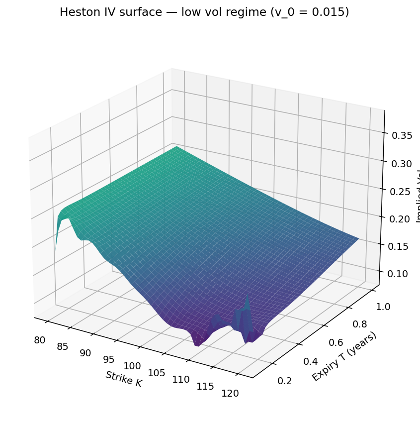

Heston IV surface at v_0 = 0.015 — low vol regime, surface sits near the bottom of the cube

$v_0 = 0.015$ (vol $\approx 12\%$). The surface sits in the bottom half of the cube, tilted left from $\rho = -0.72$. ATM IV climbs gently with $T$ as the model mean-reverts up to $\sqrt{\theta} \approx 26.5\%$.

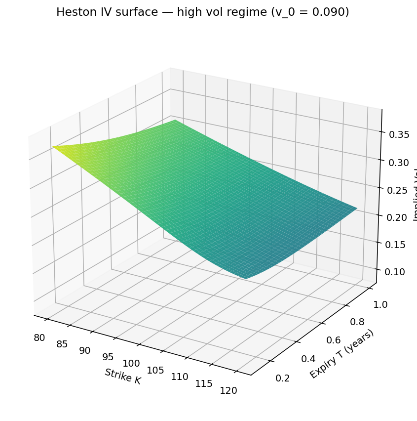
Heston IV surface at v_0 = 0.090 — high vol regime, on the same z-axis, surface is much higher up

Same z-axis. $v_0 = 0.090$ (vol $\approx 30\%$). The whole surface lifts upward — short-dated vol is now above the long-run level, and the term structure slopes down toward $\sqrt{\theta}$ as $T$ grows. Skew direction is preserved (rho hasn't changed), only the level.

Reading the dynamics off the two pictures:

$v_0$ shifts the whole surface vertically. Same shape, different height. That's the breathing you see in the reel at the top.
The term-structure slope flips sign across $\sqrt{\theta}$. Below it, ATM vol climbs with $T$ (regime is calm, but the model expects mean reversion up). Above it, ATM vol falls with $T$ (regime is stressed, mean reversion pulls down).
Skew is set by $\rho$, not by $v_0$. Both surfaces tilt the same direction and roughly the same amount. The whole reason for $\rho$ is that this asymmetry doesn't come for free from variance dynamics alone — you have to put it in by hand.
Curvature is set by $\xi$. Both surfaces have the same wing curvature even though $v_0$ is very different. If you cranked $\xi$ from $0.75$ to $1.5$ both surfaces would bow out more aggressively.

Put together: Black-Scholes gives you a single point. Heston gives you a five-parameter surface that can match observed skew, smile curvature, and term structure — and one of those five parameters ($v_t$) actually evolves through time, which is why the surface breathes.

10. Recap

Heston = Black-Scholes with the variance promoted to its own SDE.
$\rho$ controls skew direction. Negative $\rho$ = equity vol leverage effect = OTM puts richer than OTM calls.
$\xi$ controls smile curvature. Higher $\xi$ = fatter tails = more bowed wings.
$\kappa, \theta$ describe how variance reverts to its long-run level. They set the term-structure shape.
$v_0$ is today's variance state. It shifts the whole surface up or down without changing skew or curvature.
BS prices off a single point. Heston prices off a five-parameter surface that can match what the market actually quotes.

Pair this notebook with the Black-Scholes IV calculator, the gamma surface notebook, and the option Greeks notebook to see the same surface from different angles. Heston is the natural place to go after gamma — once you've stared at a BS surface long enough to feel the limits of the flat-vol assumption, the stochastic vol generalisation stops feeling like math and starts feeling like a fix for an honest gap in the model.

Free download

Get the full Heston notebook + 4 extras

Everything on this page packaged as a runnable Jupyter notebook, plus content that didn't fit here. Join the newsletter (free) and the download is yours.

The full notebook — every formula, every plot, every Python cell from this page, ready to run.
Multi-panel parameter sweep — all 4 Heston params side by side, on the same axes, for direct visual comparison.
Monte Carlo $v_t$ path simulator — 10 simulated paths overlaid with the deterministic mean, so you can see the variance distribution.
BS vs Heston pricing-difference plotter — exactly where Black-Scholes mis-prices, and by how much, across strikes and expiries.
Interactive Plotly Heston surface — rotate, zoom, hover-for-values version of the static plots above.

Write your name and a valid email to unlock the download.

heston_vol_surface_extras.ipynb

Enter your name & email above to unlock

Download

Free. One short email when there's something new. No spam, unsubscribe in one click.