
Deep hedging replaces the Black-Scholes delta formula with a neural network that learns the hedge directly. This page goes deep on the two pieces that matter: the hedge curve (the math of delta, and how it bends with price and volatility) and the tail risk (how to compute CVaR). Pure numpy and matplotlib, step by step.
Classic hedging is a formula. You sell an option, compute its Black-Scholes delta, and trade the underlying to stay delta-neutral. Deep hedging throws out the formula and lets a neural network learn the hedge directly: at each step it reads the state (price, volatility, and its own current position) and outputs how much to trade. It is trained on simulated paths to minimise a risk measure of the terminal profit and loss, including trading costs:
$$\min_{\theta}\;\; \mathrm{CVaR}_{\alpha}\!\left(-Z + \sum_t \delta_t\,\Delta S_t - C_T(\delta)\right), \qquad \delta_t = f_\theta(\log S_t,\, v_t,\, \delta_{t-1})$$
Based on the paper. This walkthrough reproduces, in a self-contained and illustrative way, the ideas from Deep Hedging by Bühler, Gonon, Teichmann and Wood (2018). For the visual intuition see the companion reel on Instagram.
Before any network, you have to understand the object it is learning. So this page goes deep on two things: the hedge curve (the math of delta, and how it moves with price and volatility) and the tail risk (how to compute CVaR).
The hedge ratio is a derivative. If $V(S)$ is the option value and $S$ the underlying price, the amount of underlying you hold to neutralise small price moves is delta:
$$\delta \;=\; \frac{\partial V}{\partial S}$$
For a European call under Black-Scholes (take the rate $r = 0$ for clarity) this derivative has a clean closed form. It is just the normal CDF evaluated at $d_1$:
$$\delta \;=\; N(d_1), \qquad d_1 \;=\; \frac{\ln(S/K) + \tfrac12\,\sigma^2\tau}{\sigma\sqrt{\tau}}$$
where $N(\cdot)$ is the standard normal CDF, $K$ the strike, $\sigma$ the volatility, and $\tau$ the time to expiry. Notice that exactly two inputs move $d_1$, and therefore the hedge: the price $S$ and the volatility $\sigma$. The whole curve is those two knobs. In code it is four lines:
import numpy as np, math

def ncdf(x):                         # standard normal CDF, N(.)
    return 0.5 * (1 + np.vectorize(math.erf)(np.asarray(x) / math.sqrt(2)))

def call_delta(S, vol, tau, K=100.0):
    d1 = (np.log(S / K) + 0.5 * vol**2 * tau) / (vol * np.sqrt(tau))
return ncdf(d1) # delta = N(d1)Fix the volatility and sweep the price. The hedge traces the classic S-curve: deep out of the money you hold almost nothing ($\delta \to 0$), deep in the money you hold one full unit ($\delta \to 1$), and at the money you sit near $\tfrac12$. The slope of this curve is gamma, the option’s second derivative:
$$\Gamma \;=\; \frac{\partial \delta}{\partial S} \;=\; \frac{N'(d_1)}{S\,\sigma\sqrt{\tau}} \;>\; 0$$
Gamma is largest at the money and near expiry, which is exactly where the curve is steepest. High gamma means the hedge changes fast for small moves in $S$, so you have to re-trade often, and re-trading is what costs money. That tension is the whole reason deep hedging exists.
import matplotlib.pyplot as plt

K, TAU = 100.0, 15 / 250          # 15 trading days to expiry
S = np.linspace(88, 112, 240)

for vol in (0.15, 0.25, 0.35):
    plt.plot(S, call_delta(S, vol, TAU), label=f"sigma = {vol:.0%}")
plt.axvline(K, ls=":", color="grey")
plt.xlabel("Price S"); plt.ylabel("hedge delta = N(d1)")
plt.legend(); plt.show()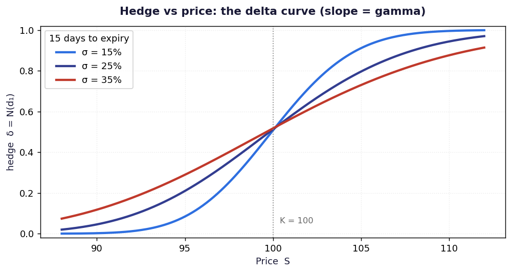
The delta curve across price, at three volatility levels. Each is an S-curve from 0 to 1, crossing near $\delta = 0.5$ at the strike. The slope is gamma. Lower volatility (blue) makes the curve steeper, that is more gamma, more re-trading, more cost.
Now fix the price and sweep the volatility. This is the part people forget: the hedge moves even when the price does not. Higher volatility pulls every delta toward $\tfrac12$, because a wider distribution makes it more uncertain which side of the strike you will finish. The sensitivity of delta to volatility is vanna:
$$\text{vanna} \;=\; \frac{\partial \delta}{\partial \sigma} \;=\; -\,N'(d_1)\,\frac{d_2}{\sigma}, \qquad d_2 = d_1 - \sigma\sqrt{\tau}$$
The sign tells the story. Out of the money ($S < K$) we have $d_2 < 0$, so vanna is positive: more volatility raises the hedge. In the money ($S > K$) vanna is negative: more volatility lowers it. At the money $d_2 \approx 0$ and the hedge barely moves. A network that only saw price would miss this entire axis.
V = np.linspace(0.05, 0.55, 240)

for S0, label in [(96, "OTM (S = 96)"), (100, "ATM (S = 100)"), (104, "ITM (S = 104)")]:
    plt.plot(V, call_delta(S0, V, TAU), label=label)
plt.axhline(0.5, ls=":", color="grey")
plt.xlabel("Volatility sigma"); plt.ylabel("hedge delta = N(d1)")
plt.legend(); plt.show()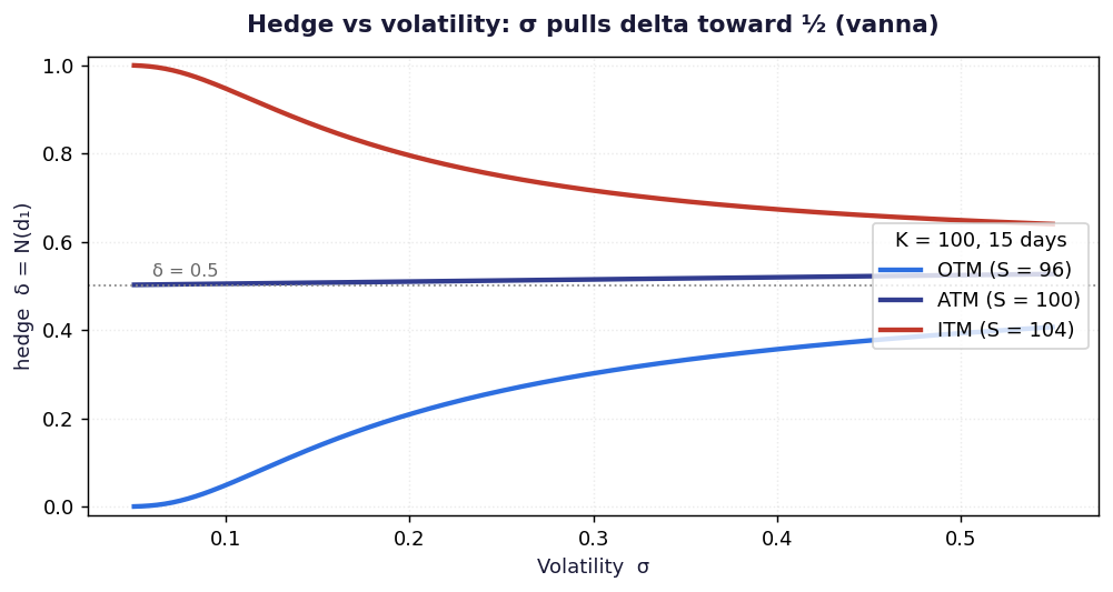
The hedge across volatility, at three price points. The out-of-the-money hedge (blue) rises toward $\tfrac12$, the in-the-money hedge (red) falls toward $\tfrac12$, and the at-the-money hedge (purple) stays flat. Volatility is a real hedging input, not just a pricing one.
The two curves above are just slices. Plot $\delta(S, \sigma)$ over both axes at once and you get the full hedge surface. This is the object the deep-hedging network learns, and it is exactly where it earns its keep: once trading costs are real, the optimal policy stops sitting on this surface at all times and instead carves a no-trade band around it, only re-hedging when it drifts too far. The formula gives you the surface; deep hedging gives you when to actually move.
from matplotlib import cm

S_ax = np.linspace(88, 112, 60); V_ax = np.linspace(0.08, 0.50, 60)
SS, VV = np.meshgrid(S_ax, V_ax)
DELTA = call_delta(SS, VV, TAU)

ax = plt.figure(figsize=(8, 5)).add_subplot(projection="3d")
ax.plot_surface(SS, VV, DELTA, cmap=cm.coolwarm)
ax.set_xlabel("Price S"); ax.set_ylabel("Volatility")
ax.set_zlabel("hedge delta"); plt.show()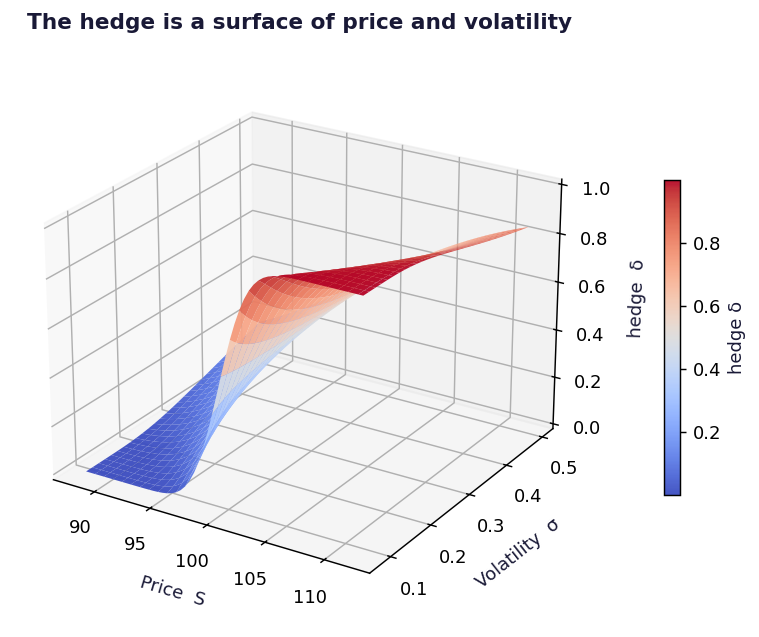
The hedge as a surface of price and volatility. The price axis is the S-curve from section 2a; the volatility axis is the pull-toward-one-half from section 2b. The deep-hedging network learns this whole map, and how it should bend once costs are real.
A real book is rarely one option. Subtract two call deltas and you get the hedge for a call spread (here, long the 98 call, short the 102 call). Its hedge surface is no longer a 0-to-1 ramp, it is a ridge that peaks between the strikes, the shape you saw rotating in the reel. Same $N(d_1)$ building block, just combined:
from matplotlib import cm

def spread_delta(S, vol, tau, KA=98.0, KB=102.0):
    return call_delta(S, vol, tau, KA) - call_delta(S, vol, tau, KB)

SPREAD = spread_delta(SS, VV, TAU)
ax = plt.figure(figsize=(8, 5)).add_subplot(projection="3d")
ax.plot_surface(SS, VV, SPREAD, cmap=cm.coolwarm)
ax.set_xlabel("Price S"); ax.set_ylabel("Volatility")
ax.set_zlabel("hedge delta"); plt.show()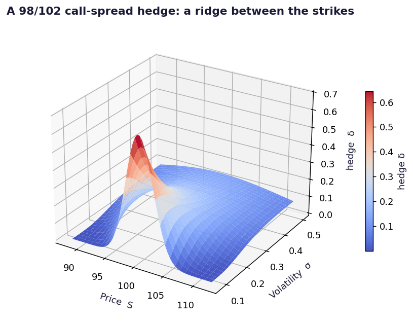
The 98/102 call-spread hedge. Instead of a 0-to-1 ramp it is a ridge that peaks between the strikes and fades outside them. The hedge ratio across price (the cross-section) is the bump you saw spinning in the video.
Everything above used the Black-Scholes formula. Deep hedging does the opposite, it never sees a formula. We give a small neural network only simulated price paths and a single instruction, minimise the risk of your final P&L, and let it discover the hedge by gradient descent.
Simulate many GBM paths of the stock. At each step the network reads the state (log-moneyness and time to expiry) and outputs a hedge ratio $\delta_t$. Tally the hedged P&L on every path and train to minimise its variance. Because the hedge enters the P&L linearly, the gradient is clean:
$$\text{P\&L} = \text{premium} - Z + \sum_t \delta_t\,\Delta S_t,\qquad \mathcal{L} = \mathrm{Var}(\text{P\&L}),\qquad \frac{\partial \mathcal{L}}{\partial \delta_t} = \frac{\partial \mathcal{L}}{\partial \text{P\&L}}\,\Delta S_t$$
(MLP below is a standard small numpy network: two hidden layers, a sigmoid output
so the hedge sits in $[0,1]$, and Adam. The novel part is the objective, not the net.)
rng = np.random.default_rng(0)
M, N, S0, K, SIG, T = 6000, 20, 100.0, 100.0, 0.20, 30/250
dt = T / N

# simulate GBM stock paths
Z = rng.standard_normal((M, N))
S = np.empty((M, N + 1)); S[:, 0] = S0
S[:, 1:] = S0 * np.exp(np.cumsum((-0.5*SIG**2)*dt + SIG*np.sqrt(dt)*Z, axis=1))
dS = S[:, 1:] - S[:, :-1]
payoff = np.maximum(S[:, -1] - K, 0.0)

# state the network sees at each step: log-moneyness and time-to-maturity
tau  = T - np.arange(N) * dt
logm = np.log(S[:, :-1] / K)
X = np.stack([logm.ravel(), np.broadcast_to(tau, (M, N)).ravel()], axis=1)

net = MLP([2, 24, 24, 1])                 # small net, sigmoid output in (0,1)
for epoch in range(400):
    d    = net.forward(X).reshape(M, N)   # hedge ratio at every (path, step)
    pnl  = premium - payoff + (d * dS).sum(axis=1)
    loss = pnl.var()                      # the ONLY objective. no delta formula.
    grad = (2 * (pnl - pnl.mean()) / M)[:, None] * dS      # dLoss/dd
    net.backprop(grad.reshape(-1, 1))     # Adam step through the network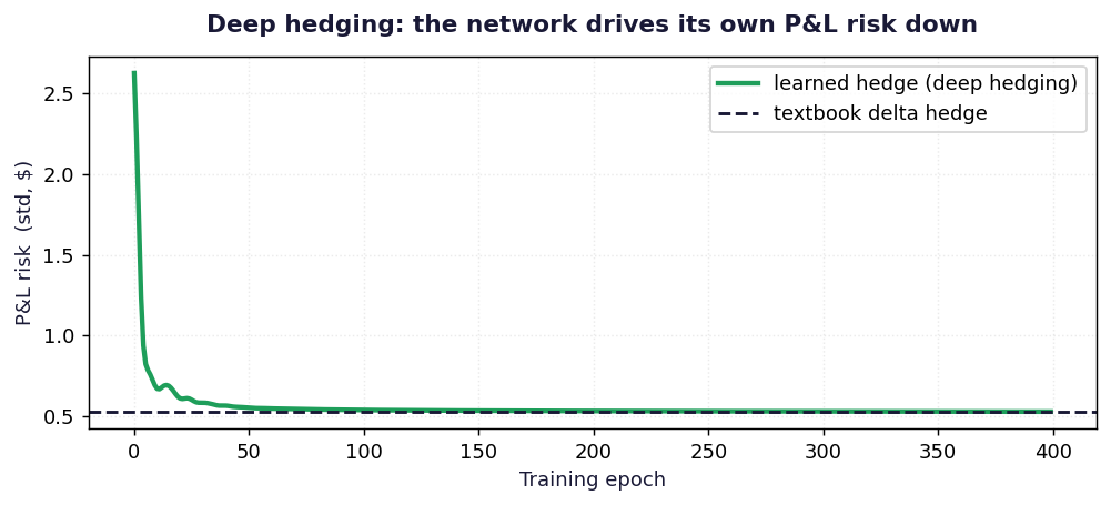
Training from random weights, the network drives its P&L risk from about $2.6 down to $0.53, right onto the dashed line, which is the risk of a textbook delta hedge on the same paths. It taught itself to hedge from paths and an objective alone.
And what did it actually learn? Plot the trained network’s hedge across price and lay the Black-Scholes delta on top. They sit on each other. The network rediscovered the delta with no formula, just paths and “minimise risk.”
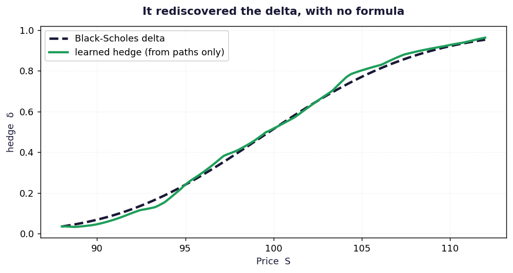
The learned hedge (green) versus the Black-Scholes delta (dashed). They match. This is the point of deep hedging: it recovers the textbook answer when the textbook is right. Add transaction costs to the objective and it stops matching, it carves a no-trade band and only re-hedges when the drift is worth the fee. That deviation is the whole payoff, and it is what the reel animates.
Deep hedging does not minimise variance, it minimises the tail. Two risk numbers describe that tail. Value at Risk is a quantile of the loss: the level the loss will not exceed with probability $\alpha$. Conditional Value at Risk (also called Expected Shortfall) goes one step further and averages the losses beyond that point, the mean of the worst $1-\alpha$ of outcomes:
$$\mathrm{CVaR}_\alpha(X) \;=\; -\,\mathbb{E}\!\left[\,X \mid X \le q_{1-\alpha}\,\right], \qquad q_{1-\alpha} = \text{the } (1-\alpha)\text{ quantile of P\&L } X$$
CVaR is what a desk actually loses on a bad day, and unlike VaR it is sensitive to how bad the tail gets, not just where it starts. Computing it from a sample of P&L outcomes is three lines: find the quantile, keep everything at or below it, average it.
rng = np.random.default_rng(5)
N = 24_000

# Terminal P&L of the book across scenarios ($k): deep hedge ON vs OFF
pnl_on  = rng.normal(0.4, 1.05, N)
pnl_off = rng.normal(0.15, 1.45, N) + rng.binomial(1, 0.06, N) * rng.normal(-3.3, 1.2, N)

def var_cvar(x, a=0.99):
    q    = np.percentile(x, (1 - a) * 100)   # the (1 - a) quantile of P&L
    var  = -q                                # Value at Risk
    cvar = -x[x <= q].mean()                  # average loss beyond it
    return round(var, 1), round(cvar, 1)

print("deep hedge ON :  VaR/CVaR =", var_cvar(pnl_on))
print("deep hedge OFF:  VaR/CVaR =", var_cvar(pnl_off))

plt.hist(pnl_off, 60, alpha=0.55, label="deep hedge OFF")
plt.hist(pnl_on,  60, alpha=0.80, label="deep hedge ON")
plt.xlabel("Terminal P&L ($k)"); plt.legend(); plt.show()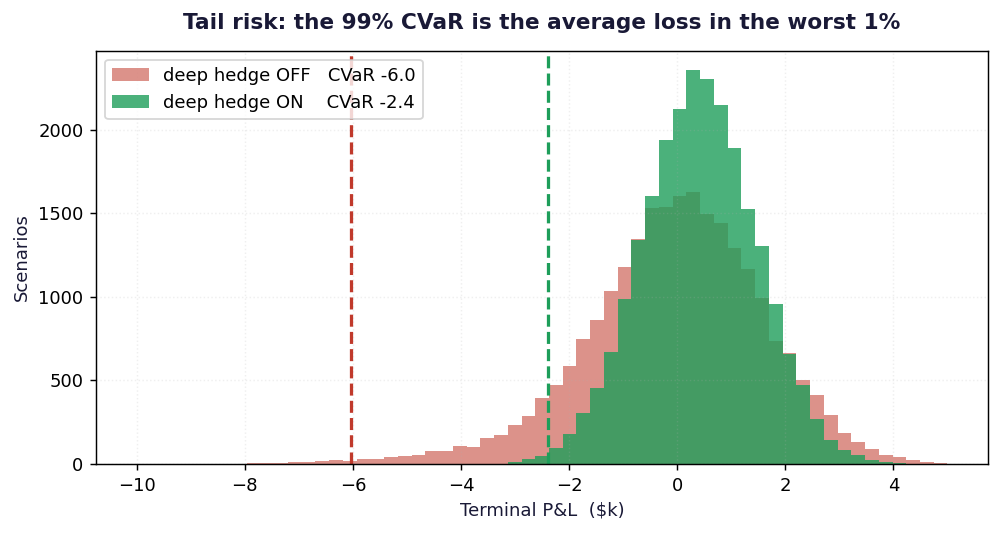
The terminal P&L distribution over thousands of scenarios. With the deep hedge on (green) the 99% CVaR is about -2.4; with it off (red) the tail fattens and the CVaR blows out to about -6.0. The dashed lines mark each CVaR. Minimising that green tail is literally the network’s training objective.
Pair this with the neural network vol surface notebook to see the same idea, a network learning a financial object directly from data, applied to the volatility smile instead of the hedge.
Everything on this page as a runnable Jupyter notebook, plus a full backtest of the learned hedge and a transaction-cost version that learns a no-trade band. Pure numpy, runs offline. Join the newsletter (free) and the download is yours.
Write your name and a valid email to unlock the download.
deep_hedging_extras.ipynb
Enter your name & email above to unlock
Free. One short email when there's something new. No spam, unsubscribe in one click.

I post the models as I build them, the changes I make to them, and the results that did not work. Shorter than these write ups, and there are a lot more of them.
Follow me on X