
Pull a live SPY option chain from yfinance, build the empirical implied volatility surface, then train two MLPs from scratch on it. Pure numpy, real Adam backprop. Watch the surface emerge over epochs, and see how network capacity decides what gets captured.
An implied volatility surface is a 2D function. Strike $K$ and time to expiry $T$ go in, an implied volatility number comes out. The market quotes one surface for every liquid underlying every minute the exchange is open, and you can pull a snapshot from yfinance in a single API call.
The question this notebook answers: can a small neural network with no built in knowledge of Black Scholes, no smile parametrisation, no SVI fit, just a stack of ReLU layers and Adam, learn the SPY vol surface from raw quotes? And if so, how much capacity does it actually need?
We train two MLPs side by side. Both see the same data, both use the same optimiser, the same learning rate, the same five input features. The only difference is the size:
Then we snapshot the prediction surface at three checkpoints to watch each one learn in slow motion.
Heads up. The results below depend entirely on the data you pull. Different days, different underlyings, different liquidity. A network that fits SPY beautifully today may give a rougher fit on TLT tomorrow. The point of this notebook is to demonstrate that the model can learn a surface and to see how it behaves epoch by epoch. It is not a backtest. There is no train, validation, test split here, because doing it properly needs a long history of option chains and most free APIs only expose the live snapshot.
Five libraries. yfinance gives us the option chain. numpy handles
the MLP forward and backward passes. pandas cleans the chain into a tidy
(K, T, IV) long format table. scipy.interpolate.griddata
interpolates that scattered point cloud onto a regular grid for visualization.
matplotlib renders the surfaces.
pip install yfinance numpy pandas scipy matplotlibimport math
from datetime import datetime, timezone
import yfinance as yf
import numpy as np
import pandas as pd
import matplotlib.pyplot as plt
from matplotlib import cm
from scipy.interpolate import griddata
yfinance exposes the option chain via two calls: Ticker.options returns the
list of available expiry dates, and Ticker.option_chain(date) returns a tuple
of (calls, puts) dataframes. Each row has a strike, a last price, a bid and
ask, volume, open interest, and yfinance’s precomputed implied volatility.
We pull the spot price first (today’s close), then loop the first 18 expiries. For each contract we keep the rows where the IV looks real (between 5% and 100%), there is some signal of liquidity (volume or open interest), and the last trade was at least a dime. Below that, the quotes get noisy. Then we filter to the OTM side at each strike: calls above spot, puts below it. That is the canonical IV surface convention. Keeping only the OTM side avoids the put call IV divergence that creeps in for ITM contracts.
# 1. Spot
tk = yf.Ticker("SPY")
S0 = float(tk.history(period="2d", auto_adjust=False)["Close"].iloc[-1])

# 2. Loop the front-of-curve expiries and collect (T, K, side, IV) rows.
rows, now = [], datetime.now(timezone.utc)
for exp_str in tk.options[:18]:
    exp_dt = datetime.strptime(exp_str, "%Y-%m-%d").replace(tzinfo=timezone.utc)
    T = (exp_dt - now).total_seconds() / (365.25 * 86400)
    if not (0.02 < T < 1.5):
        continue
    chain = tk.option_chain(exp_str)
    for side, df in [("call", chain.calls), ("put", chain.puts)]:
        df = df[(df["impliedVolatility"] > 0.05) & (df["impliedVolatility"] < 1.0)]
        df = df[(df["volume"] > 0) | (df["openInterest"] > 0)]
        df = df[df["lastPrice"] > 0.10]
        for _, r in df.iterrows():
            rows.append({"T": T, "K": float(r["strike"]),
                         "side": side, "iv": float(r["impliedVolatility"])})

chain = pd.DataFrame(rows)

# 3. Keep only OTM side at each strike (the canonical IV-surface convention).
chain = chain[((chain["side"] == "call") & (chain["K"] >= S0)) |
              ((chain["side"] == "put")  & (chain["K"] <= S0))]
# 4. Median over duplicates at the same (K, T).
chain = chain.groupby(["K", "T"], as_index=False)["iv"].median()
Now we drop the scattered (K, T, IV) triplets onto a regular 40×28 grid using
griddata. Cubic interpolation gives us a smooth surface where strikes are
dense, and nearest neighbour fills in the corners where data is sparse. Clip the result to
a readable Z range (10% to 45% IV is where SPY actually lives) so the smile structure pops
instead of getting flattened by a few outlier wings.
# Build the visualization grid: K from 85% to 115% of spot, T from 3% to 40% year.
MN_LO, MN_HI = 0.85, 1.15
T_LO,  T_HI  = 0.03, 0.40
N_K, N_T     = 40, 28

K_axis = np.linspace(MN_LO * S0, MN_HI * S0, N_K)
T_axis = np.linspace(T_LO, T_HI, N_T)
K_grid, T_grid = np.meshgrid(K_axis, T_axis)

pts  = chain[["K", "T"]].values
vals = chain["iv"].values

# Cubic where possible, nearest where sparse.
SURFACE = griddata(pts, vals, (K_grid, T_grid), method="cubic")
fill    = griddata(pts, vals, (K_grid, T_grid), method="nearest")
SURFACE = np.where(np.isnan(SURFACE), fill, SURFACE)
SURFACE = np.clip(SURFACE, 0.10, 0.45)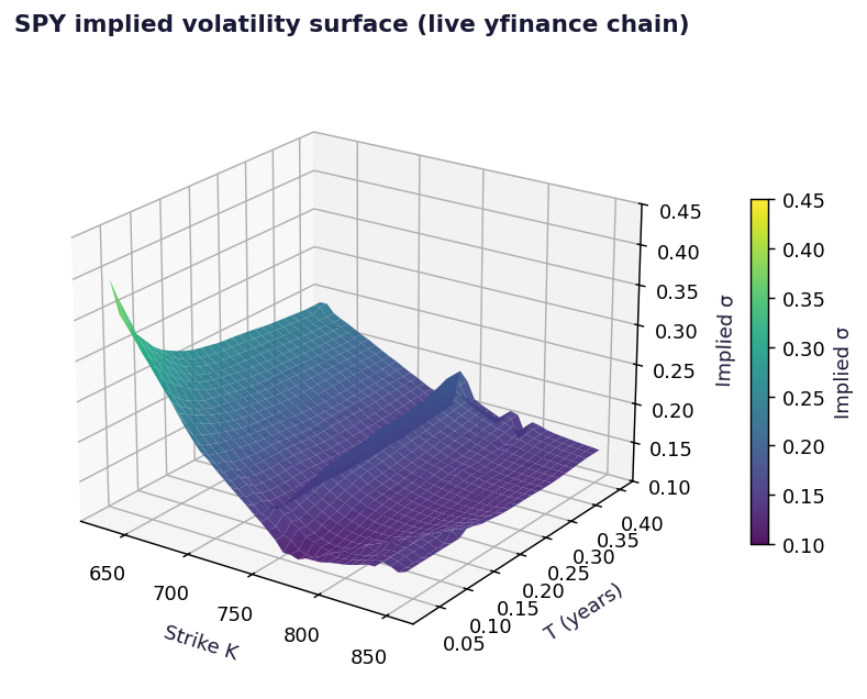
The real SPY implied volatility surface. Short dated OTM puts (front left) trade well above 30% IV. Classic equity skew. ATM short dated options (front center) sit closest to 10 to 15%. As maturity grows, the smile flattens out toward the long run vol level. This is the “truth” the network has to learn.
The network input is intentionally minimal. We give it five polynomial features built from moneyness $m = K / S_0$ and time to expiry $T$:
$$\mathbf{x} = (\, m,\; T,\; m^2,\; T^2,\; m\,T \,)$$
No log moneyness, no SVI parametrisation, no Black Scholes structure baked in. Just raw polynomial interactions. If the network is going to learn a smile, it has to discover the $m^2 / T$ shape on its own. That is the whole point of the experiment.
Then we standardize the features (zero mean, unit variance) and center the IV target around its mean. Both are standard tricks that make gradient descent behave: features on the same scale prevent any single one from dominating the gradient, and a centered target keeps the bias terms from doing all the work in early epochs.
def features(K, T, S0):
    K = np.asarray(K).flatten()
    T = np.asarray(T).flatten()
    m = K / S0
    return np.stack([m, T, m**2, T**2, m * T], axis=1)

X_full = features(K_grid, T_grid, S0)
y_full = SURFACE.flatten().reshape(-1, 1)

# Standardize features, center the target.
X_mean = X_full.mean(axis=0, keepdims=True)
X_std  = X_full.std(axis=0, keepdims=True) + 1e-9
X_norm = (X_full - X_mean) / X_std

Y_MEAN     = float(y_full.mean())
y_centered = y_full - Y_MEANNo PyTorch, no TensorFlow. Just a plain Python class that stores weights, runs a forward pass with ReLU activations on the hidden layers, and does the backward pass with the Adam optimiser. That means first and second moment estimates of the gradient, bias corrected for the warmup steps.
Why Adam and not vanilla SGD? Because Adam is the de facto default for small data MLP fitting and because it converges fast enough that we can show meaningful progress in 600 epochs without playing with the learning rate. The weights are He initialised ($\sigma = \sqrt{2 / n_{\text{in}}}$) so the variance of the activations does not collapse through the layers.
class MLP:
    """Feedforward MLP with ReLU activations + Adam optimizer.  Pure numpy."""

    def __init__(self, sizes, seed=42):
        rng = np.random.default_rng(seed)
        self.sizes = sizes
        self.W, self.b = [], []
        self.mW, self.mb, self.vW, self.vb = [], [], [], []
        for i in range(len(sizes) - 1):
            std = math.sqrt(2.0 / sizes[i])                    # He init
            self.W.append(rng.standard_normal((sizes[i], sizes[i + 1])) * std)
            self.b.append(np.zeros((1, sizes[i + 1])))
            self.mW.append(np.zeros_like(self.W[-1]))
            self.mb.append(np.zeros_like(self.b[-1]))
            self.vW.append(np.zeros_like(self.W[-1]))
            self.vb.append(np.zeros_like(self.b[-1]))
        self.t = 0   # Adam timestep counter

    def forward(self, X):
        activations, z_values = [X], []
        a = X
        for i, (W, b) in enumerate(zip(self.W, self.b)):
            z = a @ W + b
            z_values.append(z)
            # ReLU on hidden layers; linear output.
            a = np.maximum(0, z) if i < len(self.W) - 1 else z
            activations.append(a)
        return a, activations, z_values

    def backward(self, y, activations, z_values, lr,
                 beta1=0.9, beta2=0.999, eps=1e-8):
        self.t += 1
        m = y.shape[0]
        delta = 2 * (activations[-1] - y) / m                 # MSE grad
        for i in reversed(range(len(self.W))):
            a_prev = activations[i]
            dW = a_prev.T @ delta
            db = delta.sum(axis=0, keepdims=True)
            if i > 0:
                delta = (delta @ self.W[i].T) * (z_values[i - 1] > 0)
            # Adam moments
            self.mW[i] = beta1 * self.mW[i] + (1 - beta1) * dW
            self.mb[i] = beta1 * self.mb[i] + (1 - beta1) * db
            self.vW[i] = beta2 * self.vW[i] + (1 - beta2) * dW * dW
            self.vb[i] = beta2 * self.vb[i] + (1 - beta2) * db * db
            mW_hat = self.mW[i] / (1 - beta1 ** self.t)
            mb_hat = self.mb[i] / (1 - beta1 ** self.t)
            vW_hat = self.vW[i] / (1 - beta2 ** self.t)
            vb_hat = self.vb[i] / (1 - beta2 ** self.t)
            self.W[i] -= lr * mW_hat / (np.sqrt(vW_hat) + eps)
self.b[i] -= lr * mb_hat / (np.sqrt(vb_hat) + eps)Two architectures, same training loop. 600 epochs, learning rate 0.02. At specific checkpoint epochs we save the current prediction surface so we can visualize how each network is doing.
SMALL_LAYERS = [5,   4,   4, 1]          #     49 parameters
BIG_LAYERS   = [5, 128, 128, 1]          # 17,409 parameters
EPOCHS       = 600
LR           = 0.02
CHECKPOINTS  = [0, 50, 200, 600]

def train_with_snapshots(layers):
    mlp = MLP(layers, seed=42)
    losses = []
    snaps  = {}
    for epoch in range(EPOCHS + 1):
        y_pred, activs, zs = mlp.forward(X_norm)
        loss = float(np.mean((y_pred - y_centered) ** 2))
        losses.append(loss)
        if epoch in CHECKPOINTS:
            snaps[epoch] = (y_pred.flatten() + Y_MEAN).reshape(SURFACE.shape)
        if epoch < EPOCHS:
            mlp.backward(y_centered, activs, zs, LR)
    return snaps, np.array(losses)

small_snaps, small_losses = train_with_snapshots(SMALL_LAYERS)
big_snaps, big_losses = train_with_snapshots(BIG_LAYERS)Same plotting routine, applied to each saved snapshot. The white wireframe overlay on each chart is the true SPY surface (the “target”), and the colored surface underneath is the network’s current prediction.
At epoch 50, both networks have caught the average level of the surface. They predict a flattish IV around 18 to 22%. The BIG net is starting to bend, the SMALL net is still mostly a plane.
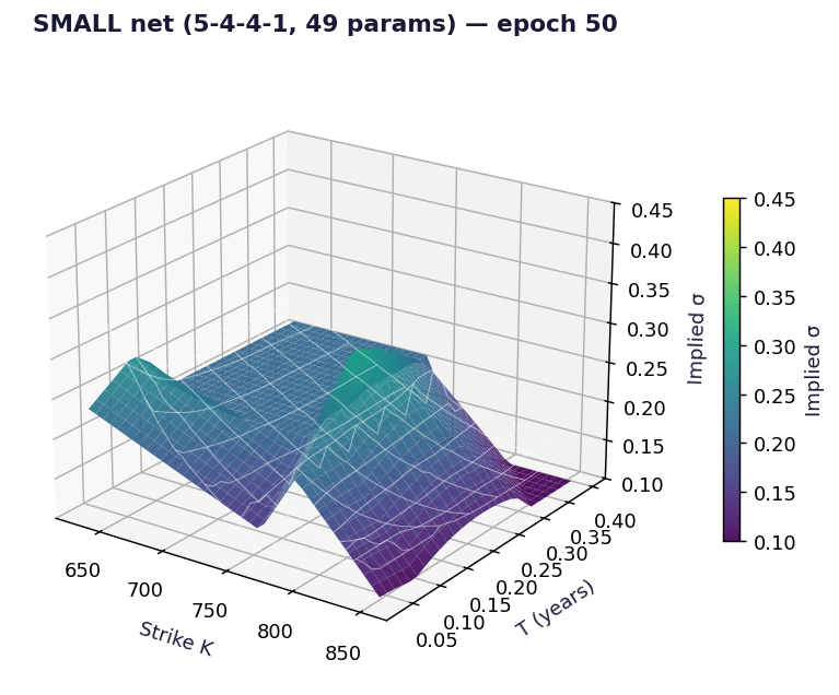
SMALL net at epoch 50. Predicts the surface mean, doesn’t yet have the moneyness curvature.
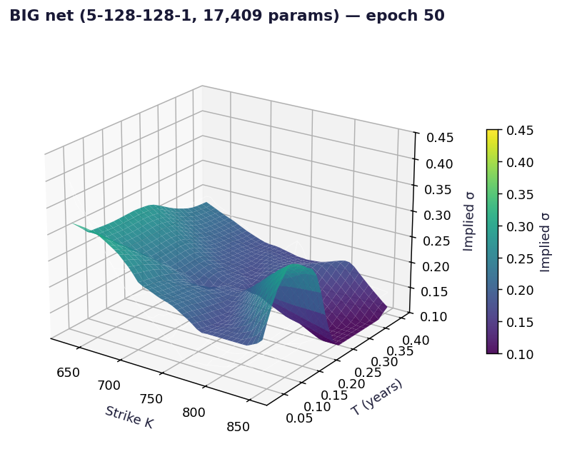
BIG net at epoch 50. Starting to bend at the OTM put wing. The skew is emerging.
At epoch 200, both networks now have a smile shape. The BIG net is close to the truth in most places, including the steep front left OTM put corner. The SMALL net has the right general shape but lacks the resolution to capture the corner curl.
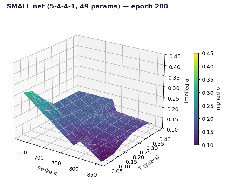
SMALL net at epoch 200. The smile is there but blunted at the OTM put wing.
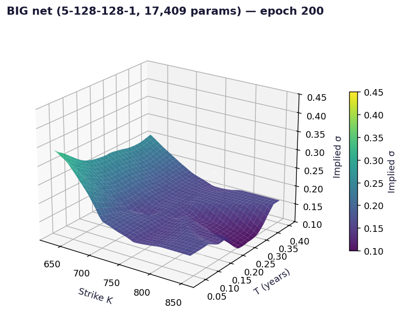
BIG net at epoch 200. Almost on top of the truth wireframe across the full grid.
At epoch 600, training is done. The BIG net’s prediction is essentially indistinguishable from the truth wireframe. The SMALL net is also “close”, but the deep OTM put corner stays blunt. It does not have enough hidden units to bend that sharply.
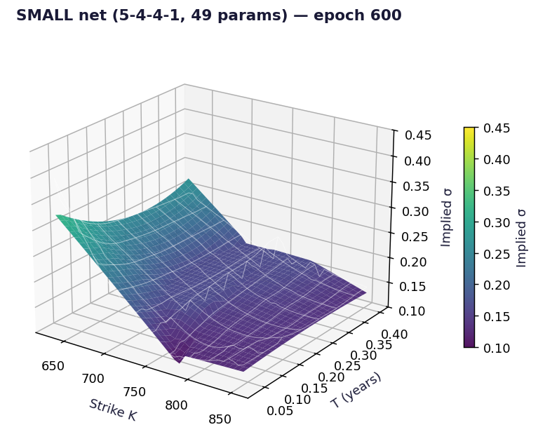
SMALL net at epoch 600. Final training RMSE around 1.0%. Capacity limited at the corner.
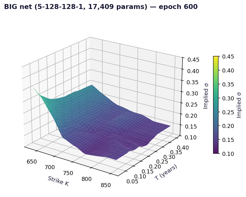
BIG net at epoch 600. Final training RMSE around 0.76%. The surface is fully captured.
The story of those snapshots, in one chart. Y axis is training RMSE on a log scale (because epoch 0 starts at 100% and converges to under 1%). Both networks crash through the same trajectory for the first 80 epochs or so, learning the smile’s mean level and rough skew. After that they separate. The BIG net keeps shaving off error well past epoch 300, the SMALL net flattens.
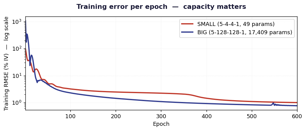
Training RMSE per epoch on a log scale. Both networks converge fast for the first 80 epochs, then diverge. The SMALL net plateaus around 1% RMSE, the BIG net keeps improving to about 0.76%. The gap is small in absolute terms, but it is exactly the corner of the surface that matters most for OTM put pricing.
SPY for TLT, QQQ, NVDA, anything liquid.Pair this with the Heston vol surface notebook. That is the parametric, financial math approach to the same problem. Heston says: the smile must come from these five SDE parameters. The neural network says: I don’t need a theory, give me the data. Both end up with a surface that fits the market. The choice is whether you want interpretability or flexibility.
Everything on this page packaged as a runnable Jupyter notebook, plus a fully interactive 3D version of the surface that goes beyond the walkthrough. Join the newsletter (free) and the download is yours.
Write your name and a valid email to unlock the download.
neural_network_vol_surface_extras.ipynb
Enter your name & email above to unlock
Free. One short email when there's something new. No spam, unsubscribe in one click.

I post the models as I build them, the changes I make to them, and the results that did not work. Shorter than these write ups, and there are a lot more of them.
Follow me on X