Gamma Surface in Python | David Arias, CFA

Watch the Greeks walkthrough

Before diving into the surface, here's my 15-minute video that builds intuition for all four first-order Greeks (Delta, Gamma, Theta, Vega) and explains how the gamma surface animation in this notebook was put together. It also covers the third-order Greeks (Zomma, Color, Speed) referenced near the end of this page. Click to play right here.

1. What gamma is, in one sentence

Gamma is the rate at which the option's delta changes when the underlying moves by one dollar. Delta tells you how the option price moves; gamma tells you how that movement itself accelerates or decelerates as the stock drifts away from where it is now.

It is the same number for calls and puts, it is always non-negative, and it is at its largest when the option is at the money. The further you go in or out of the money, the less responsive delta becomes, so gamma fades to zero.

The closed-form expression from Black-Scholes is:

$$\Gamma \;=\; \frac{\varphi(d_1)}{S\,\sigma\,\sqrt{T}}, \qquad d_1 \;=\; \frac{\ln(S/K) + (r + \tfrac{1}{2}\sigma^2)\,T}{\sigma\sqrt{T}}$$

where $\varphi$ is the standard normal density. That is the only formula on this page. Everything that follows is just slicing this expression along a different axis to see what moves it.

2. Setup

Three libraries are enough: numpy for the maths, scipy for the standard normal, and matplotlib for the plots. Install them once if you don't have them:

pip install numpy scipy matplotlib

Then the imports and the closed-form gamma function used by every cell below.

import numpy as np
from scipy.stats import norm
import matplotlib.pyplot as plt
from matplotlib import cm

def d1(S, K, T, r, sigma):
    return (np.log(S / K) + (r + 0.5 * sigma ** 2) * T) / (sigma * np.sqrt(T))

def gamma(S, K, T, r, sigma):
    return norm.pdf(d1(S, K, T, r, sigma)) / (S * sigma * np.sqrt(T))

# Defaults we will reuse below
S0, K0, T0, R0, SIG0 = 100.0, 100.0, 0.5, 0.05, 0.25

3. Gamma vs Spot price

Hold everything constant and move the underlying. Gamma traces a bell shape that peaks near the strike and dies off in both directions. The peak sits a touch below the strike because the drift term $r$ pulls the centre of $d_1$ slightly to the left.

spots  = np.linspace(60, 140, 400)
gammas = gamma(spots, K0, T0, R0, SIG0)

plt.figure(figsize=(8, 4.2))
plt.plot(spots, gammas, lw=2.2)
plt.axvline(K0, color="red", ls="--", alpha=0.6, label=f"Strike K = {K0:.0f}")
plt.title(f"Gamma vs Spot price  (K={K0:.0f}, T={T0}, sigma={SIG0:.0%}, r={R0:.0%})")
plt.xlabel("Spot price S"); plt.ylabel("Gamma")
plt.legend(); plt.grid(True); plt.tight_layout(); plt.show()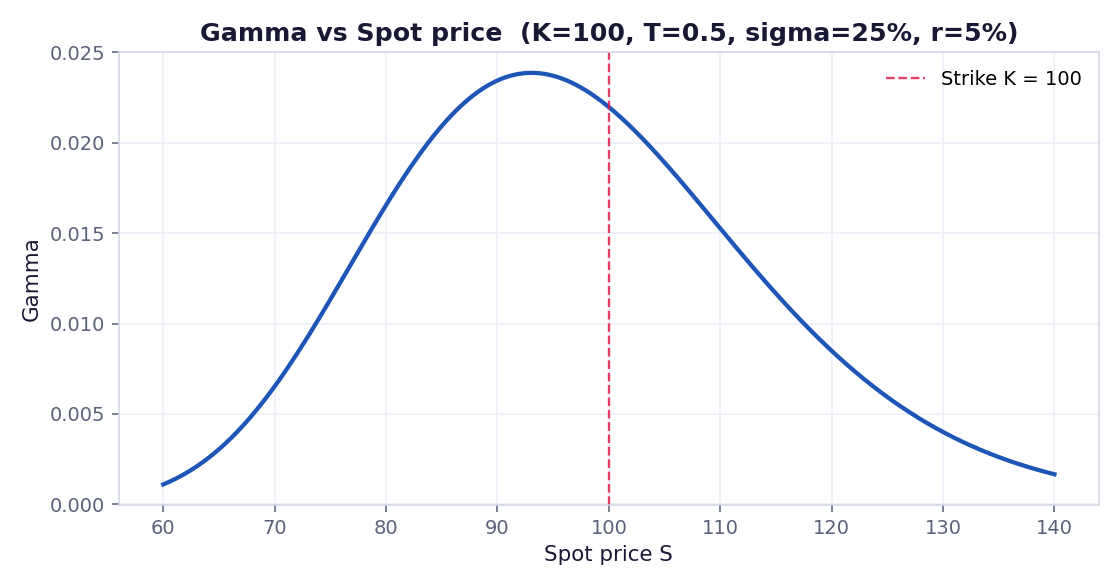

Gamma vs spot price — bell-shape peaking near the strike

Gamma is largest when the option is at the money and decays smoothly toward zero on both wings.

4. Gamma vs Volatility

Now freeze the spot at the money and sweep volatility. Gamma decreases as vol rises. Intuitively, a highly volatile stock has its delta already spread across a wide range of likely outcomes, so an extra dollar of movement at the spot doesn't change delta much. A quiet stock concentrates all of the delta near the strike, so the same dollar move flips a lot more probability mass.

vols   = np.linspace(0.05, 1.20, 400)
gammas = gamma(S0, K0, T0, R0, vols)

plt.figure(figsize=(8, 4.2))
plt.plot(vols * 100, gammas, lw=2.2)
plt.title(f"Gamma vs Volatility  (ATM: S=K={K0:.0f}, T={T0}, r={R0:.0%})")
plt.xlabel("Volatility sigma (%)"); plt.ylabel("Gamma")
plt.grid(True); plt.tight_layout(); plt.show()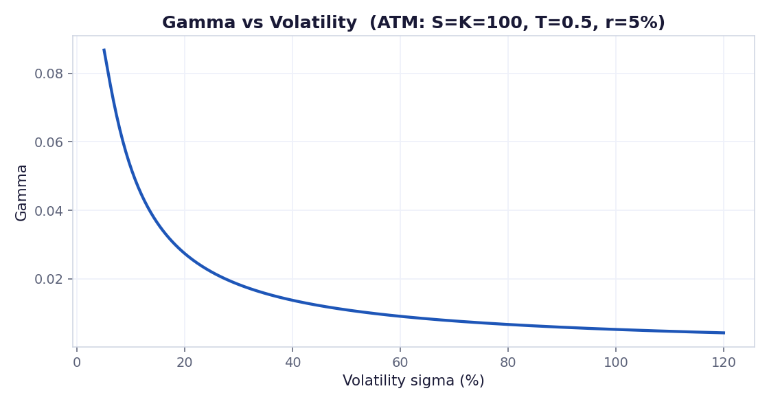

Gamma vs volatility — monotonically decreasing curve

At the money, gamma falls as volatility rises. Low-vol names carry the sharpest gamma at expiry.

5. Gamma vs Time to expiry

Same setup, only now we sweep $T$. As expiry approaches, gamma at the money does the opposite of vega: it shoots up. This is the source of the famous "gamma squeeze" stories you read about during weekly expiries on liquid names.

Far from expiry, every cent of stock movement only marginally changes the probability the option finishes in the money. Near expiry, only the last few cents around the strike still flip the outcome, so the option reacts violently in that tiny zone.

times  = np.linspace(0.01, 2.0, 400)
gammas = gamma(S0, K0, times, R0, SIG0)

plt.figure(figsize=(8, 4.2))
plt.plot(times, gammas, lw=2.2)
plt.title(f"Gamma vs Time to expiry  (ATM: S=K={K0:.0f}, sigma={SIG0:.0%}, r={R0:.0%})")
plt.xlabel("Time to expiry T (years)"); plt.ylabel("Gamma")
plt.gca().invert_xaxis()  # time flows toward expiry on the right
plt.grid(True); plt.tight_layout(); plt.show()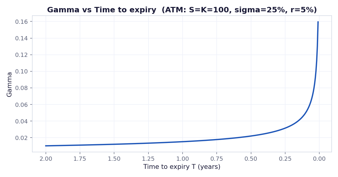

Gamma vs time to expiry — explodes near zero

Time flows from left to right. The closer we get to expiry, the sharper at-the-money gamma becomes.

6. Gamma vs Strike

Last 1D slice: fix the spot and walk the strike. The shape mirrors the spot sweep, but the peak now sits a hair above the spot rather than below. Same reason as before, just on the opposite axis: the drift in $d_1$ tilts the centre of mass.

strikes = np.linspace(60, 140, 400)
gammas  = gamma(S0, strikes, T0, R0, SIG0)

plt.figure(figsize=(8, 4.2))
plt.plot(strikes, gammas, lw=2.2)
plt.axvline(S0, color="red", ls="--", alpha=0.6, label=f"Spot S = {S0:.0f}")
plt.title(f"Gamma vs Strike  (S={S0:.0f}, T={T0}, sigma={SIG0:.0%}, r={R0:.0%})")
plt.xlabel("Strike K"); plt.ylabel("Gamma")
plt.legend(); plt.grid(True); plt.tight_layout(); plt.show()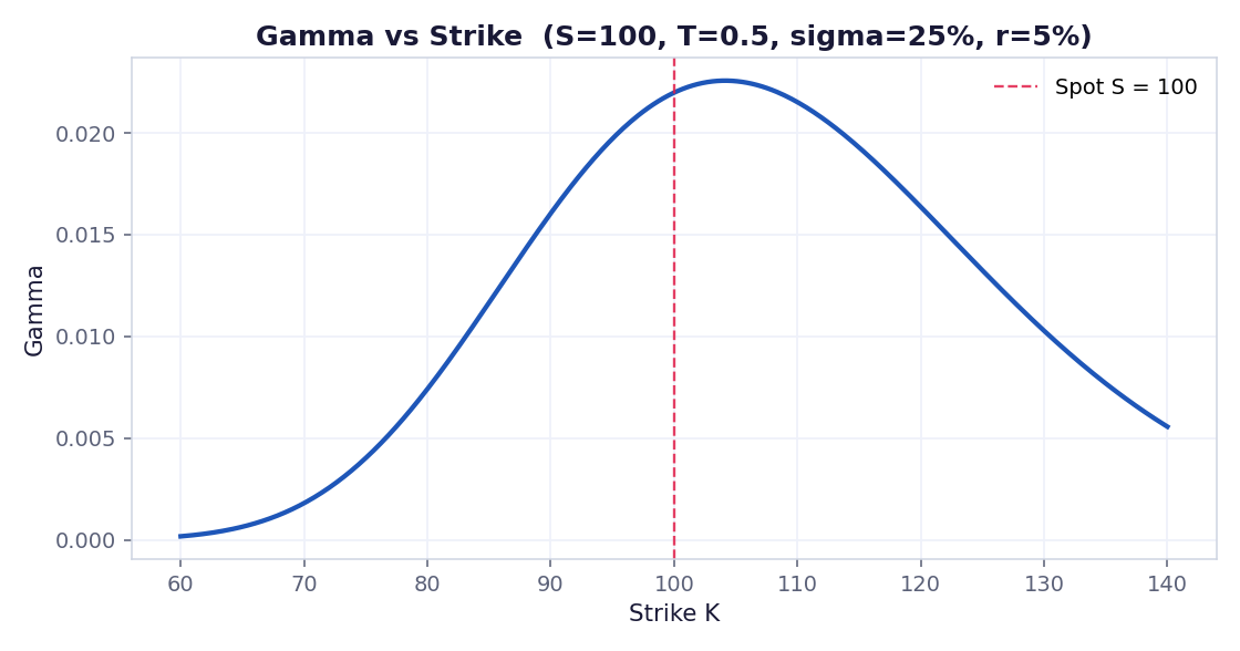

Gamma vs strike — bell-shape peaking just above the spot

Walking the strike across a fixed spot produces the mirror picture of section 3.

7. Stacking it all: the gamma surface

With the four 1D slices in hand, the 3D surface stops feeling abstract. Put moneyness $K/S$ on one floor axis, volatility $\sigma$ on the other, and let the height of the surface be gamma. Every cell so far is just one slice through this object.

The trick to reading the surface is to compare two snapshots taken at different times-to-expiry on the same z-scale. The two plots below use identical axis ranges and the identical colour mapping. Whatever moves between them is what time does to gamma, with nothing else changed.

moneyness = np.linspace(0.70, 1.30, 90)   # K/S
vols      = np.linspace(0.10, 0.80, 80)
M, V = np.meshgrid(moneyness, vols)
K_grid    = M * S0                          # strikes implied by moneyness * spot

# Compute BOTH surfaces first so we can share the z-axis and colour scale
G_long  = gamma(S0, K_grid, 0.30, R0, V)    # ~3.5 months to expiry
G_short = gamma(S0, K_grid, 0.10, R0, V)    # ~5 weeks to expiry
Z_MAX   = max(G_long.max(), G_short.max()) * 1.02

for T_FIXED, G_surf in [(0.30, G_long), (0.10, G_short)]:
    fig = plt.figure(figsize=(9, 6.2))
    ax  = fig.add_subplot(111, projection="3d")
    ax.plot_surface(M, V * 100, G_surf, cmap=cm.viridis, edgecolor="none",
                    alpha=0.95, vmin=0, vmax=Z_MAX)   # shared colour scale
    ax.set_zlim(0, Z_MAX)                              # shared z-axis
    ax.set_title(f"Gamma surface at T = {T_FIXED}  (S={S0:.0f}, r={R0:.0%})")
    ax.set_xlabel("Moneyness K/S"); ax.set_ylabel("Volatility sigma (%)")
    ax.set_zlabel("Gamma")
    ax.view_init(elev=22, azim=-58)
    plt.tight_layout(); plt.show()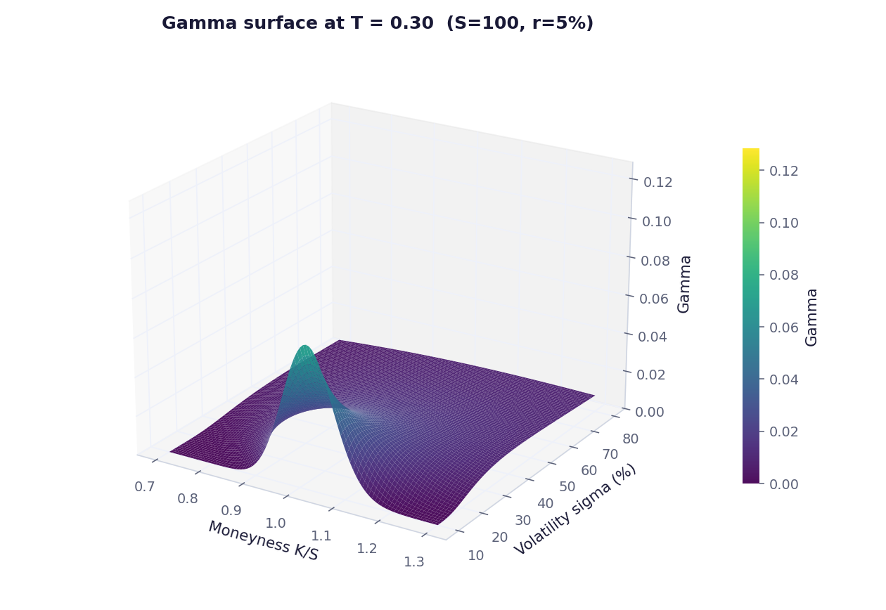

Black-Scholes gamma surface at T = 0.30 — moderate ridge at ATM, low vol

$T = 0.30$. The surface sits low in the cube. The peak is in the ATM, low-vol corner but only reaches about a third of the z-axis. Colours are mostly cool — there's almost no yellow anywhere.

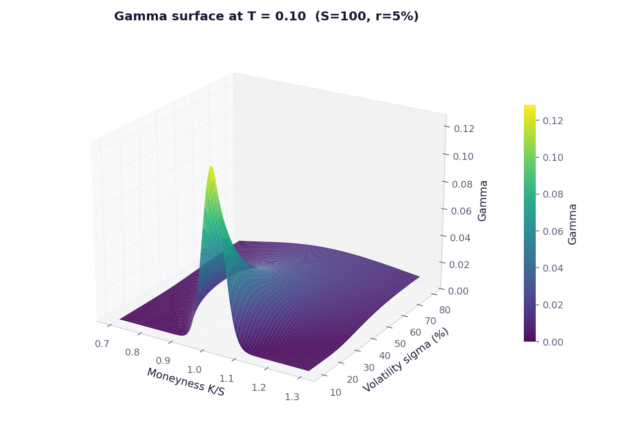
Black-Scholes gamma surface at T = 0.10 — tall sharp spike at ATM, low vol

$T = 0.10$ on the exact same z-axis. The peak now reaches the top of the cube and turns bright yellow on the colour bar. Everywhere else on the surface barely moved. All of the action concentrates at the ATM low-vol corner.

Reading the dynamics off the two pictures:

The peak is fixed in space. Moneyness $\approx 1$ on one axis, the lowest $\sigma$ on the other. That corner is the "high gamma" cell of the option surface, and it doesn't move when $T$ changes.
Only the height of that peak changes. From the formula $\Gamma = \varphi(d_1) / (S \sigma \sqrt{T})$, the $\sqrt{T}$ in the denominator shrinks as $T$ shrinks, so the gamma at that corner blows up. The other corners barely move because the $\varphi(d_1)$ numerator is already near zero there.
The vol axis controls how wide the ridge is. A low-vol underlying ($\sigma \approx 10\%$) compresses all of the delta near the strike, so the ridge is narrow and tall. A high-vol underlying ($\sigma \approx 80\%$) spreads delta across a wide moneyness band, so the ridge is broad and flat.
The "gamma cliff" is the slope you walk from spot to slightly OTM. On the $T = 0.10$ surface the wall around the peak is almost vertical — that's why a small move in spot can swing your delta dramatically near expiry.

You can keep playing with these numbers. Try $T = 0.05$ or $T = 0.02$ next, the peak keeps climbing while the rest of the surface flattens. Try widening the vol range to $\sigma \in [0.05, 1.0]$ and the high-vol tail gets even flatter.

8. The gamma-theta trade-off (mirror plot)

Long gamma is the thing you want when you expect the underlying to move. The problem is it never comes for free: every dollar of gamma you carry is paid for in theta. The two Greeks are mirror opposites when you plot them against the strike at the same expiry.

Take $T = 0.15$ (roughly two months to expiry), fix the spot and the vol, and walk the strike from $60$ to $140$. Gamma traces a positive bell that peaks just above the spot. Theta traces a negative bell that troughs at the same spot. Same shape, opposite sign.

def theta_call(S, K, T, r, sigma):
    dd1 = d1(S, K, T, r, sigma)
    dd2 = dd1 - sigma * np.sqrt(T)
    return (-S * norm.pdf(dd1) * sigma / (2.0 * np.sqrt(T))
            - r * K * np.exp(-r * T) * norm.cdf(dd2))

T_MIRROR = 0.15
strikes  = np.linspace(60, 140, 400)
gammas   = gamma(S0, strikes, T_MIRROR, R0, SIG0)
thetas   = theta_call(S0, strikes, T_MIRROR, R0, SIG0) / 365.0   # negative

plt.figure(figsize=(9, 5))
plt.plot(strikes, gammas, lw=2.4, label="Gamma  (positive — gains as spot moves)")
plt.plot(strikes, thetas, lw=2.4, label="Theta per day  (negative — daily bleed)")
plt.axhline(0, color="gray", lw=0.8)
plt.axvline(S0, color="gray", lw=0.8, ls="--", label=f"Spot S = {S0:.0f}")
plt.title(f"Gamma and Theta — mirror opposites at T = {T_MIRROR}")
plt.xlabel("Strike K"); plt.ylabel("Value")
plt.legend(); plt.grid(True); plt.tight_layout(); plt.show()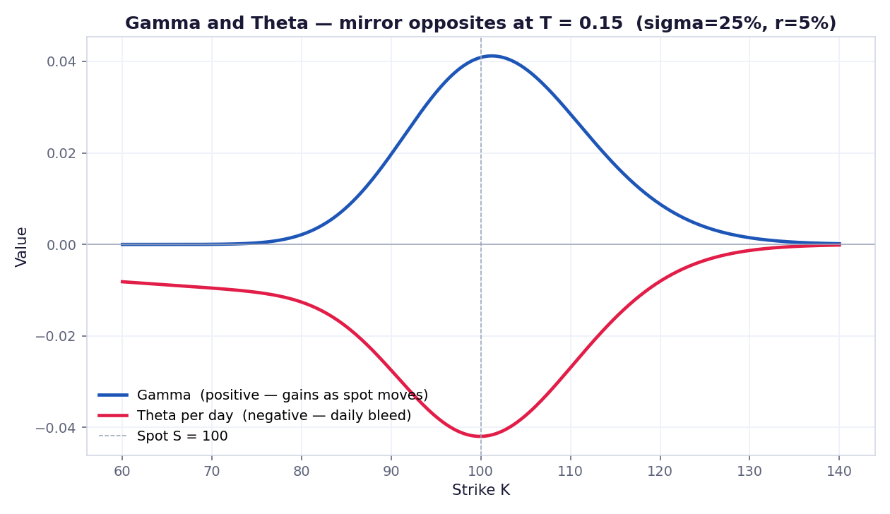

Gamma and Theta as mirror opposites at T = 0.15, plotted against Strike

The blue curve (gamma) and the red curve (theta-per-day) trace the same shape on opposite sides of zero. Both peak in magnitude right at the spot. That is the gamma- theta trade-off in one image: wherever gamma is biggest, theta is most negative. Carrying long gamma at the strike is exactly where you pay the most theta every day.

9. Two higher-order Greeks: Zomma and Vanna

Once you start thinking about how gamma itself moves when other inputs change, you've crossed into the higher-order Greeks. The two that show up most often around the gamma surface are Zomma and Vanna. Both answer the same kind of question: "what happens to my gamma exposure if implied vol moves?"

9.1 Zomma — how gamma reacts to a change in volatility

Zomma is the literal derivative of gamma with respect to $\sigma$, so it's the slope of the gamma surface along the vol axis at any given strike.

$$\text{Zomma} \;=\; \frac{\partial \Gamma}{\partial \sigma} \;=\; \Gamma \cdot \frac{d_1\,d_2 - 1}{\sigma}$$

It is negative right at the strike (a vol uptick flattens the gamma peak) and positive in the wings (the same vol uptick lifts gamma OTM and ITM, because options that were too far out of the money to have meaningful gamma now start to react). That sign flip is the key intuition.

def zomma(S, K, T, r, sigma):
    dd1 = d1(S, K, T, r, sigma)
    dd2 = dd1 - sigma * np.sqrt(T)
    return gamma(S, K, T, r, sigma) * (dd1 * dd2 - 1.0) / sigma

T_3 = 0.15
strikes = np.linspace(60, 140, 400)
gamma_curve = gamma(S0, strikes, T_3, R0, SIG0)
zomma_curve = zomma(S0, strikes, T_3, R0, SIG0)

fig, ax1 = plt.subplots(figsize=(9, 4.6))
ax1.plot(strikes, gamma_curve, lw=2.4, label="Gamma  (left)")
ax1.set_xlabel("Strike K"); ax1.set_ylabel("Gamma")
ax2 = ax1.twinx()
ax2.plot(strikes, zomma_curve, color="green", lw=2.4, label="Zomma  (right)")
ax2.set_ylabel("Zomma (dGamma / dSigma)")
plt.title(f"Zomma vs Gamma at T = {T_3}"); plt.tight_layout(); plt.show()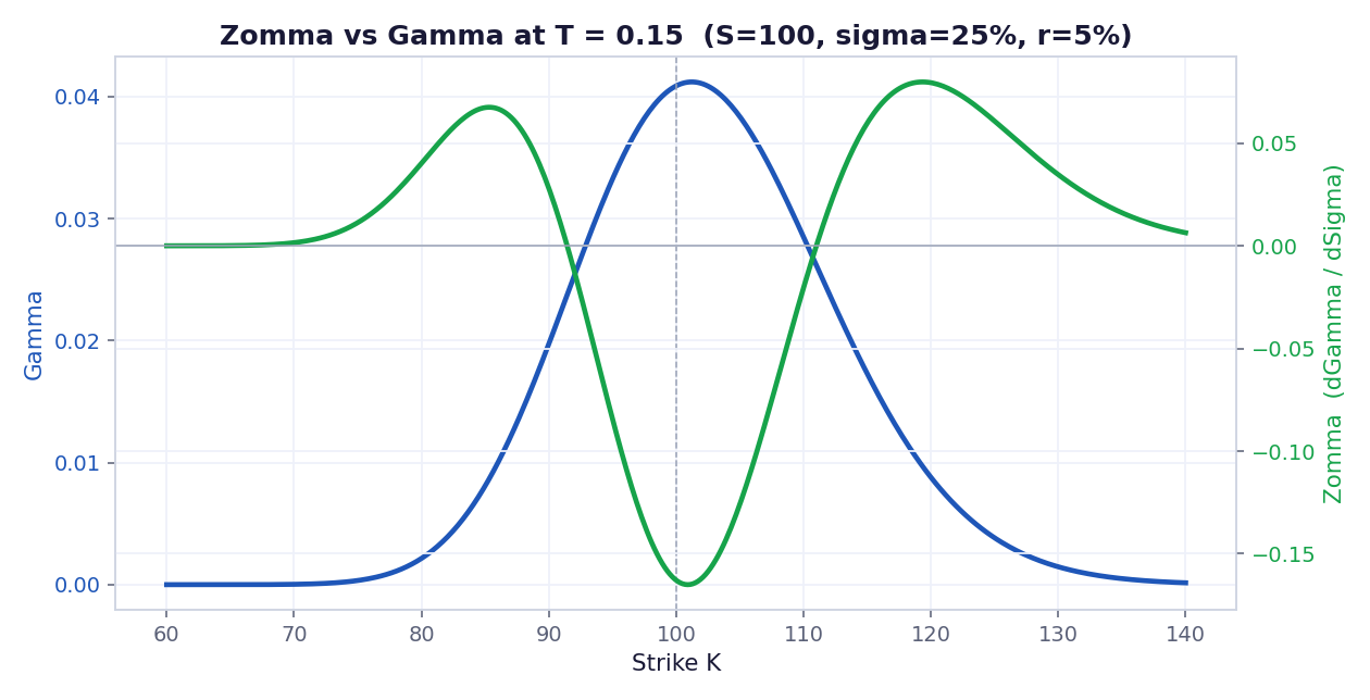

Zomma vs Gamma at T = 0.15 — Zomma is negative at the strike, positive in the wings

Blue is gamma (positive bell). Green is Zomma — it dips deep below zero exactly under the gamma peak and rises into two positive humps on either side. Reading: an increase in $\sigma$ flattens the gamma peak and lifts the wings, which is exactly how the 3D surface widens when vol rises.

9.2 Vanna — how delta reacts to a change in volatility

Vanna is one step over from Zomma: instead of asking how gamma moves with $\sigma$, it asks how delta moves with $\sigma$. Equivalently, how vega moves with spot. It is a cross-Greek between the volatility surface and the spot direction.

$$\text{Vanna} \;=\; \frac{\partial \Delta}{\partial \sigma} \;=\; \frac{\partial \mathcal{V}}{\partial S} \;=\; -\frac{\varphi(d_1)\,d_2}{\sigma}$$

Vanna is the reason your delta drifts even when the spot doesn't move. If implied vol rises, an out-of-the-money call gets more delta (positive Vanna). If implied vol drops, that delta evaporates. Vanna is most important for OTM positions, which is where gamma is small — so Vanna picks up the directional risk that gamma misses.

def vanna(S, K, T, r, sigma):
    dd1 = d1(S, K, T, r, sigma)
    dd2 = dd1 - sigma * np.sqrt(T)
    return -norm.pdf(dd1) * dd2 / sigma

vanna_curve = vanna(S0, strikes, T_3, R0, SIG0)

fig, ax1 = plt.subplots(figsize=(9, 4.6))
ax1.plot(strikes, gamma_curve, lw=2.4, label="Gamma  (left)")
ax1.set_xlabel("Strike K"); ax1.set_ylabel("Gamma")
ax2 = ax1.twinx()
ax2.plot(strikes, vanna_curve, color="purple", lw=2.4, label="Vanna  (right)")
ax2.set_ylabel("Vanna (dDelta / dSigma)")
plt.title(f"Vanna vs Gamma at T = {T_3}"); plt.tight_layout(); plt.show()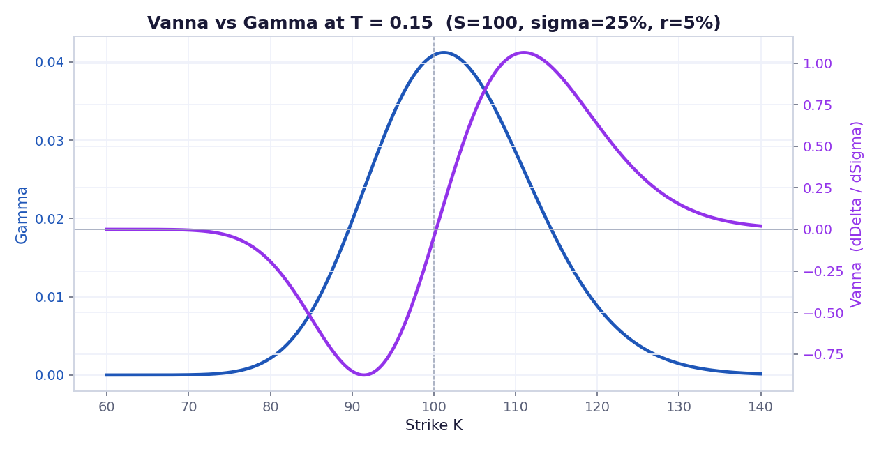

Vanna vs Gamma at T = 0.15 — Vanna crosses zero at the strike

Vanna crosses zero at the strike (where gamma peaks) and is negative for ITM strikes, positive for OTM strikes. That sign profile is why a vol rally helps OTM call buyers (positive Vanna) and hurts ITM call sellers — even before the spot actually moves. Gamma at the same strikes is essentially zero, so Vanna is the Greek doing the work in those wings.

Zomma and Vanna both belong to the family of "vol-of-gamma" Greeks. Gamma alone tells you what one spot move does to your option. Zomma and Vanna tell you what a volatility move does to that gamma exposure — which is exactly the kind of risk that shows up when an earnings release or a Fed meeting reprices the whole vol surface in seconds. The longer walk-through (Speed, Color, Ultima) is in the YouTube video at the top of the page.

10. Recap

Gamma peaks at the money and decays smoothly into both wings.
At fixed spot, higher volatility means lower gamma at the money.
At fixed vol, gamma at the money explodes as $T \to 0$.
On the surface, the peak's location is fixed (ATM, low vol). Only the peak's height changes with $T$.
Gamma and theta are mirror opposites against strike at fixed expiry. Long gamma is paid for in theta.
Zomma tells you how gamma reacts to a vol move. Vanna tells you how delta reacts to a vol move.

Once you have this surface in your head, half of options trading lore (gamma scalping, weekly pin risk, the dealer gamma flip) reduces to: "where on this surface are we, and which direction is the spot pushing us?"

Pair this notebook with the Greeks calculator or the full Greeks notebook to see the other Greeks in the same setup.