
Feed forward, recurrent, convolutional, transformer and autoencoder, each built in PyTorch and pointed at a job it is actually suited for. A live SPY option chain, twenty years of daily returns, and 45 US large caps. Free data throughout, splits by date, and one result that did not survive a rerun.
Trees stop somewhere. Machine learning for equity and fixed income ran decision trees, random forests and XGBoost over a stock panel, and left neural networks out on purpose, because a network only earns its cost when the data has a shape a tree cannot see. Sequences have that shape. So do pictures, and so does a smile across strikes. This page picks up there.
Five architectures run below, in the order a course would teach them. Each one gets the task it was invented for, and a real dataset rather than a simulation:
Data comes from yfinance and nothing else. No API key, no subscription, no vendor
terminal. Option chains, twenty years of adjusted closes and a 45 name cross section all arrive
from one free source, which means every block below runs on a laptop the moment it is pasted in.
Training runs on a GPU through PyTorch and falls back to CPU on its own.
Read the limitations before quoting any number here. One result on this page is openly unstable, the universe is 45 names rather than a market, no transaction cost is charged anywhere, and two of the five correlations sit on overlapping windows. And section 6 scores every network against a baseline that costs nothing, which two of them lose to.
Ninety four firm characteristics feed a neural network with three hidden layers, trained on expanding windows so that validation never sees the future. Predictions rank every stock, then the top decile is bought and the bottom decile sold. Model selection runs on the information coefficient rather than mean squared error, which holds up better on limited data. Method comes from Gu, Kelly and Xiu (2020), Empirical Asset Pricing via Machine Learning, rebuilt here on free data instead of the 30,000 stocks and 920 features of the original. Last step connects the book to the Interactive Brokers API through a Python script, so the strategy places its own long short orders rather than printing a backtest. Code and notebook are on GitHub.
I post the models as I build them, the changes I make to them, and the results that did not work. Shorter than these write ups, and there are a lot more of them.
Follow me on X


Sections below walk through each network step by step, with the reasoning, the charts and the snippet that matters. Full build, both scripts end to end and every figure they produce, sits in the repository.
Plainest architecture there is. Numbers enter one side, pass through a stack of layers that each multiply, add and bend, and a number comes out the other. No memory of the previous input, no sense of order, no idea that two inputs might be neighbours. What it does have is the ability to approximate any smooth function, which is exactly the job when a surface has to be fitted through scattered quotes.
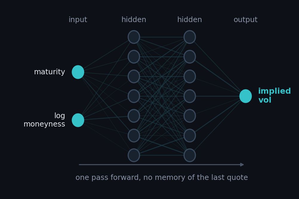
Derivatives desks use this shape constantly. A fitted surface has to be evaluated at strikes and maturities nobody quoted, and a network gives a smooth interpolant that costs microseconds to query, so an exotic book can be revalued thousands of times inside a risk run. Same trick works as a calibration surrogate: train a network to imitate a slow model such as Heston or rough Bergomi, then call the network instead of the solver. Credit and consumer lending use it too, on flat tabular applicant data, where gradient boosting is usually the tougher opponent.
Quotes come from the SPY option chain as it stands right now, first sixteen expiries. Only out of the money contracts are kept, calls above spot and puts below, because a call and a put on the same strike carry different quoted vols and feeding both teaches the network to average two different things. Filters on volume and bid drop the stale rows.
Live chain, then a three layer network on moneyness and maturity
import numpy as np, pandas as pd, yfinance as yf
import torch, torch.nn as nn

spy = yf.Ticker("SPY"); spot = float(spy.history(period="5d")["Close"].iloc[-1])
rows = []
for exp in spy.options[:16]:
    ch = spy.option_chain(exp)
    t = (pd.Timestamp(exp) - pd.Timestamp.today()).days / 365.0
    if t <= 0.02: continue
    # OTM only: calls above spot, puts below. Same strike, two different quoted vols.
    for df, side in ((ch.calls, "c"), (ch.puts, "p")):
        d = df[(df.impliedVolatility > 0.03) & (df.impliedVolatility < 1.5)
               & (df.volume > 5) & (df.bid > 0.05)]
        d = d[d.strike >= spot] if side == "c" else d[d.strike < spot]
        for k, iv in zip(d.strike, d.impliedVolatility):
            rows.append((np.log(k / spot), t, iv))

S = pd.DataFrame(rows, columns=["m", "t", "iv"])
S = S[(S.m.abs() < 0.35)].dropna()

ffn = nn.Sequential(nn.Linear(2, 96), nn.Tanh(), nn.Linear(96, 96), nn.Tanh(),
                    nn.Linear(96, 96), nn.Tanh(), nn.Linear(96, 1)).to(DEV)
opt = torch.optim.Adam(ffn.parameters(), lr=3e-3)
for ep in range(6000):
    opt.zero_grad(); ((ffn(Xn[tr]) - y[tr]) ** 2).mean().backward(); opt.step()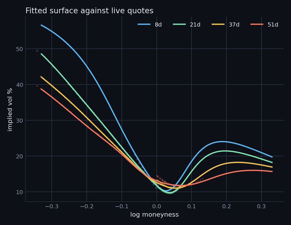
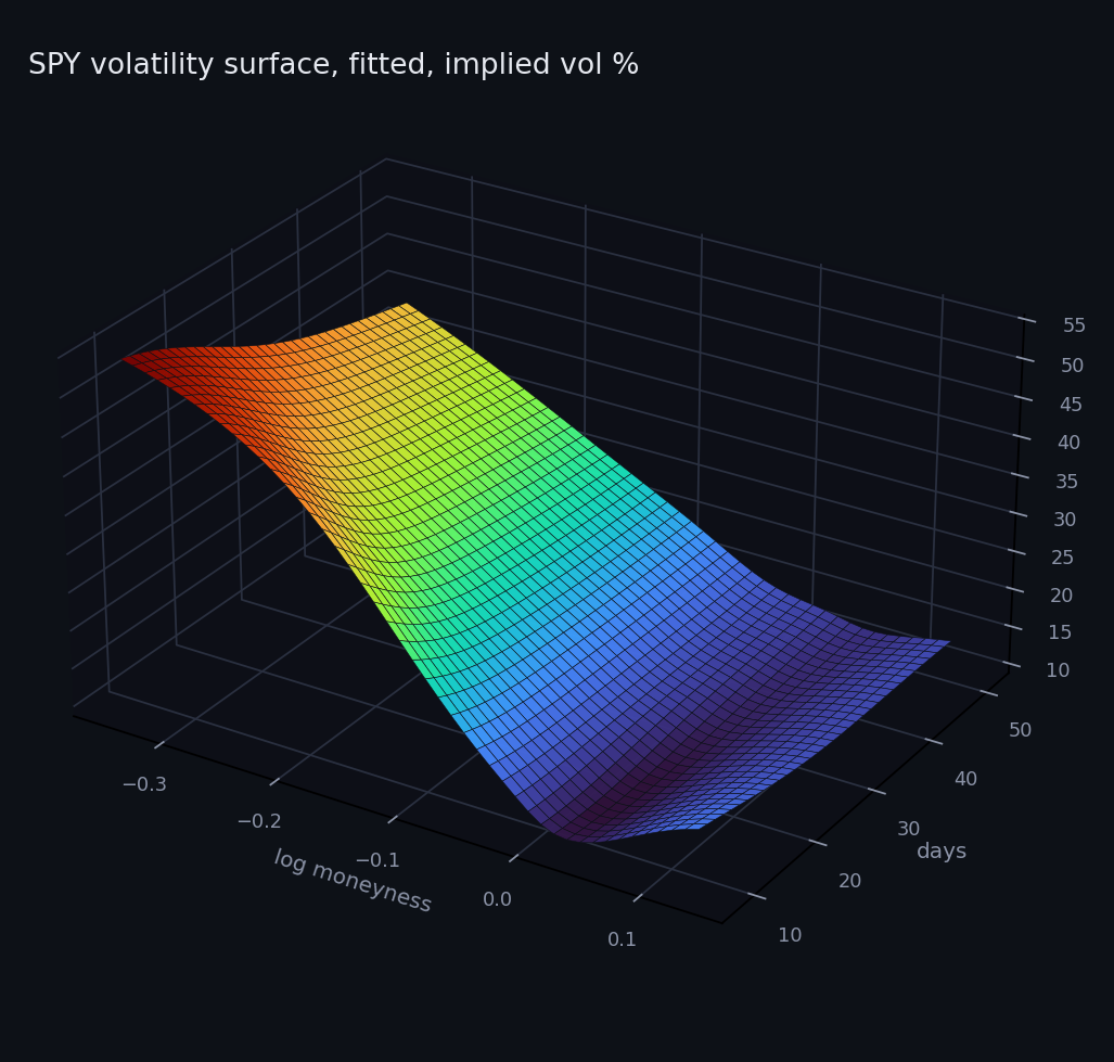
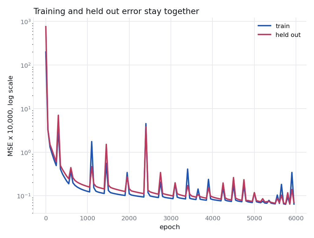
Result. 998 live quotes around a spot of 767.32, split 80/20, and a held out root mean squared error of 0.251 volatility points. Quoted vols in that chain run from roughly 10 to 55, so a quarter of a point sits inside the bid ask spread across most of the surface.
One caveat belongs to this section alone. Splitting at random is defensible here and wrong everywhere else on this page, because a surface at a single instant has no time axis to leak across. Every other model below splits by date.
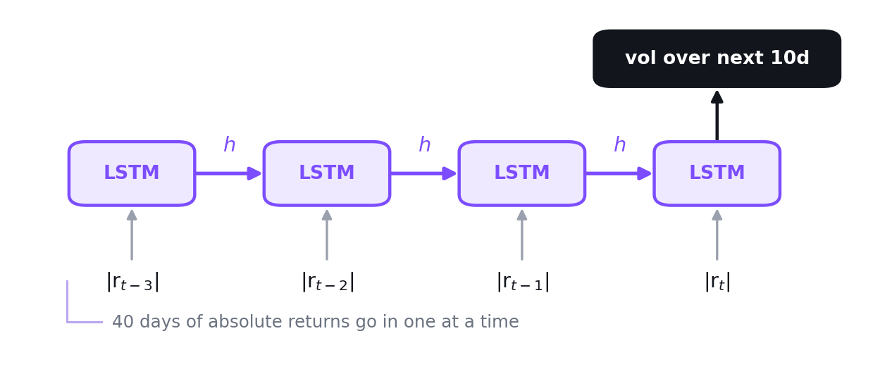
Recurrent networks read a sequence one step at a time and carry a hidden state forward, so position changes the answer. An LSTM adds gates that decide what to keep and what to drop, which is what stops the signal from a spike forty days back dissolving before it reaches the output. Order matters here, and that is the entire reason to reach for this shape.
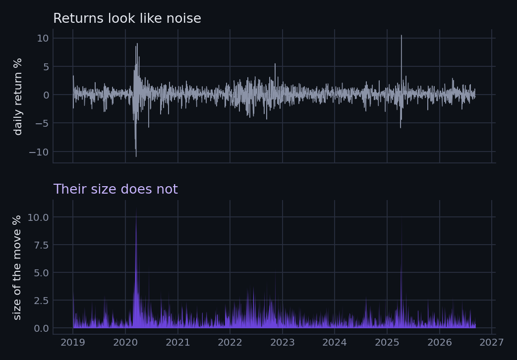
Risk management is the obvious home. Value at risk, margin and stress numbers all need a forward volatility estimate, and volatility clusters, which makes it one of the few genuinely predictable objects in markets. Volatility desks use the same forecast to judge whether an option is cheap against what is likely to be realised. Microstructure teams run sequence models over order flow, where the ordering of events carries the information. Credit uses them over payment histories, where a borrower's sequence of late payments says more than the count of them.
Input is forty days of absolute returns, annualised. Target is realised volatility over the next ten days. Split lands at 75% of the sample, so training stops in September 2021 and every scored day comes after it, including the April 2025 spike that no part of training ever saw.
One LSTM layer, 48 hidden units, fitted on the first 75% of the history
px = yf.Ticker("SPY").history(period="20y")["Close"].dropna()
r  = np.log(px / px.shift(1)).dropna()
LOOK, FWD = 40, 10

fwd_vol = r[::-1].rolling(FWD).std()[::-1].shift(-1) * np.sqrt(252)
feat    = np.abs(r.values) * np.sqrt(252)
Xs, ys  = [], []
for i in range(LOOK, len(r) - FWD - 1):
    v = fwd_vol.iloc[i]
    if np.isfinite(v):
        Xs.append(feat[i - LOOK:i]); ys.append(v)

cut = int(len(Xs) * 0.75)              # split in TIME, never shuffled

class LSTMVol(nn.Module):
    def __init__(s, h=48):
        super().__init__(); s.l = nn.LSTM(1, h, batch_first=True); s.o = nn.Linear(h, 1)
    def forward(s, x): return s.o(s.l(x)[0][:, -1])

rnn = LSTMVol().to(DEV); opt = torch.optim.Adam(rnn.parameters(), lr=2e-3)
for ep in range(400):
    opt.zero_grad(); ((rnn(Xtr) - ytr) ** 2).mean().backward(); opt.step()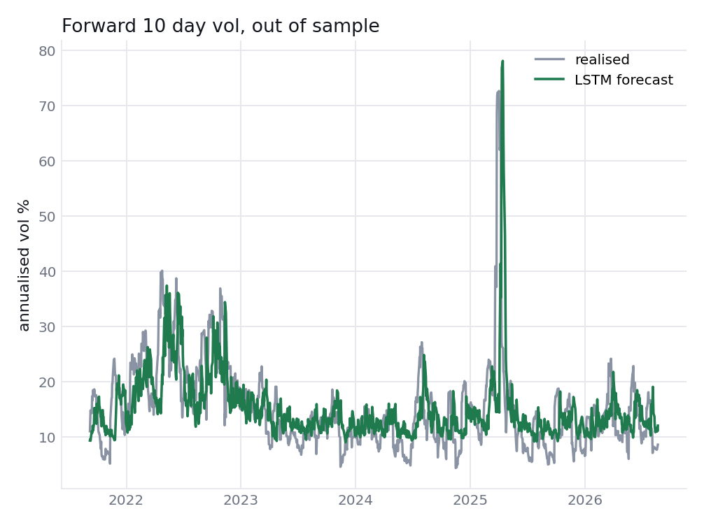
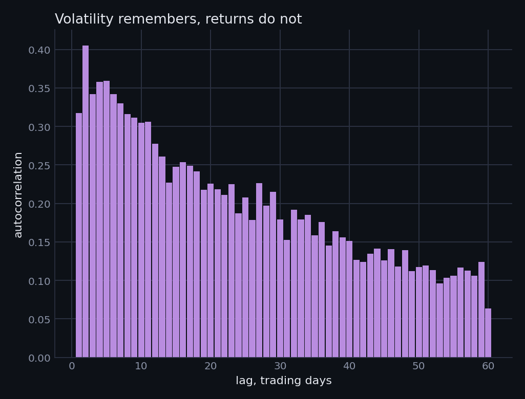
Result. 4,978 windows, out of sample from 7 September 2021, correlation 0.457 against realised volatility with a root mean squared error of 7.74 volatility points. Forecasting the level of vol is a task where 0.46 is a respectable number and a long way below the 0.9 that a persistence chart can flatter you into expecting. HAR-RV on the same windows reaches 0.53, see section 6.
Convolutional networks slide a small filter across an input and ask the same question at every position. Built for images, where a diagonal edge means a diagonal edge wherever it appears, and the layers stack so early filters find edges while later ones find combinations of edges. Applied to a price chart, that translates into something a table of returns cannot express: shape, and the relationship between a bar and its neighbours.
Idea comes from Jiang, Kelly and Xiu, (Re-)Imag(in)ing Price Trends, Journal of Finance 2023. Rather than hand engineering momentum and reversal features, draw the last twenty days as a bar chart and hand the picture to a network. Whatever technical pattern exists, the filters are free to find it, and whatever does not exist stays unfound.
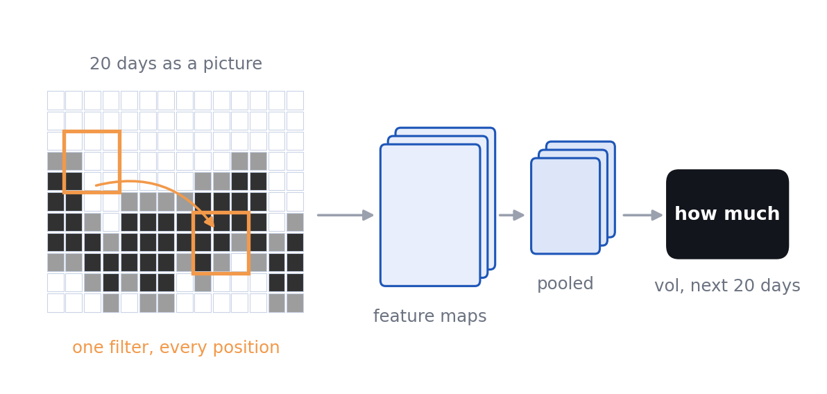
Systematic equity is the direct application, and the paper above is the reference. Beyond charts, the same architecture reads limit order book snapshots as heat maps in microstructure research, turns satellite imagery of parking lots and storage tanks into alternative data for equity research, and handles scanned documents in credit operations. Anywhere a two dimensional layout carries meaning, this is the tool.
Each image is 32 rows by 60 columns. Every day gets three columns: a tick on the left for the open, the high to low bar in the middle, a tick on the right for the close, plus a volume strip along the bottom. Prices are rescaled inside each window, so a 400 dollar stock and a 40 dollar stock produce the same picture when they move the same way. Level disappears and shape is all that survives, which is the whole point of the method.
Rendering a window, then the convolutional stack
JAN, PIX, ALTP, ALTV = 20, 3, 26, 6         # 20 days, 3 px each, 26 price rows, 6 volume rows
ALT = ALTP + ALTV

def desenha(o, h, l, c, v):
    img = np.zeros((ALT, JAN * PIX), dtype=np.float32)
    lo, hi = l.min(), h.max()
    esc = lambda p: int(np.clip((p - lo) / (hi - lo) * (ALTP - 1), 0, ALTP - 1))
    vmax = v.max()
    for d in range(JAN):
        x = d * PIX
        img[esc(o[d]), x]                       = 1.0     # open tick, left
        img[esc(l[d]):esc(h[d]) + 1, x + 1]     = 1.0     # high low bar, middle
        img[esc(c[d]), x + 2]                   = 1.0     # close tick, right
        a = int(np.clip(v[d] / vmax * ALTV, 0, ALTV))
        if a: img[ALTP:ALTP + a, x + 1] = 0.6             # volume strip
    return img[::-1]                                      # row 0 on top, like a screen

class CNN(nn.Module):
    def __init__(self):
        super().__init__()
        self.c1, self.c2   = nn.Conv2d(1, 16, (5, 3), padding=(2, 1)), nn.Conv2d(16, 32, (5, 3), padding=(2, 1))
        self.bn1, self.bn2 = nn.BatchNorm2d(16), nn.BatchNorm2d(32)
        self.fc, self.drop = nn.Linear(32 * (ALT // 4) * (JAN * PIX // 4), 1), nn.Dropout(0.4)

    def forward(self, x):
        x = F.max_pool2d(F.leaky_relu(self.bn1(self.c1(x))), 2)
        x = F.max_pool2d(F.leaky_relu(self.bn2(self.c2(x))), 2)
        return self.fc(self.drop(x.flatten(1)))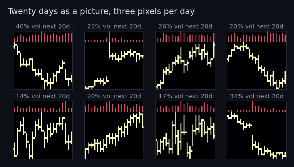
Direction is the question everyone asks first, and it is not reported here as a result. Four runs of the same code returned quintile spreads of 0.18, 0.19, 0.01 and 0.16 percentage points over twenty days, with 0.01 stored alongside this build, so how big the answer looks depends on which day fell where in the split. Classification accuracy of 0.553 says nothing either, because the label is unbalanced: over any twenty day horizon most windows on US large caps end higher, so answering "up" every single time scores about the same. Honest summary is that these images give a coin flip on direction.
Same images answer a different question well. Swap the classifier head for a regression on log realised volatility over the following twenty days, keep everything else identical, and the picture turns out to carry real information about how much a name is about to move.
Same body, regression head, target is log realised vol over the next 20 days
volnet = CNN().to(DEV)
opt = torch.optim.Adam(volnet.parameters(), lr=8e-4, weight_decay=1e-4)

lv      = torch.tensor(np.log(YV))[:, None]                  # YV = fwd 20d realised vol, %
mv, sv  = float(lv[:corte].mean()), float(lv[:corte].std())  # scaled on TRAIN only
lvn     = (lv - mv) / sv

for ep in range(10):
    for k in range(0, corte, 512):
        b = np.random.permutation(corte)[k:k + 512]
        opt.zero_grad()
        F.mse_loss(volnet(xt[b].to(DEV)), lvn[b].to(DEV)).backward()
        opt.step()

pv  = np.exp(pred * sv + mv)                                 # back to vol points
print(np.corrcoef(pv, YV[corte:])[0, 1])                     # 0.225 out of sample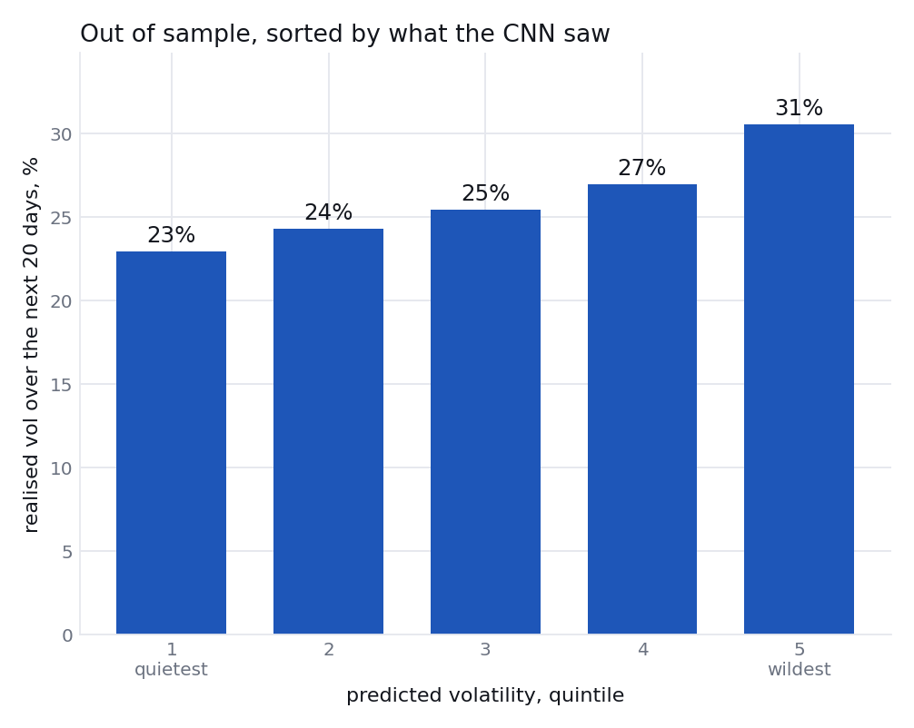
Result. 153,000 images across 45 names, out of sample from 20 March 2023, correlation 0.225 between predicted and realised volatility, and a ladder running 22.9% to 30.6% from quietest quintile to wildest. Small, and it is the kind of small that survives being looked at twice. Trailing twenty day vol on the same rows reaches 0.51, see section 6.
Transformers dropped the walk through a sequence entirely. Every position looks at every other position at once and learns how much weight to put on each, through a query, a key and a value per step. Nothing has to survive forty sequential updates to reach the output, so a spike from thirty days ago arrives at full strength if the model decides it matters. Parallel, and it scales, which is why every large language model is built on this block.
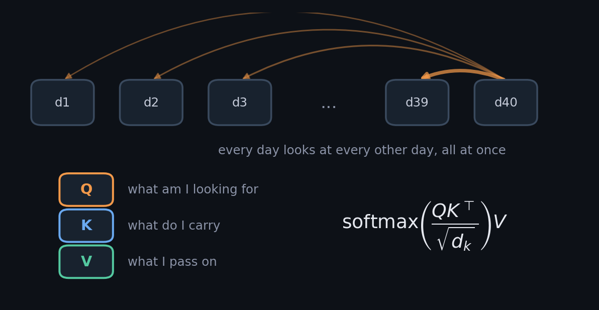
Only architecture changes here. Same forty day window, same ten day forward volatility target, same split date, same optimiser and the same 400 steps. Anything different in the answer belongs to the model.
Single head block: projection, learned positions, attention, layer norm
class Attn(nn.Module):
    def __init__(s, d=32):
        super().__init__()
        s.p   = nn.Linear(1, d)
        s.pos = nn.Parameter(torch.randn(1, LOOK, d) * 0.02)   # learned position codes
        s.a   = nn.MultiheadAttention(d, 4, batch_first=True)
        s.n   = nn.LayerNorm(d); s.o = nn.Linear(d, 1)

    def forward(s, x, want=False):
        h = s.p(x) + s.pos
        z, w = s.a(h, h, h, need_weights=want, average_attn_weights=True)
        return s.o(s.n(h + z)[:, -1]), w                       # residual, then last position

tr_ = Attn().to(DEV); opt = torch.optim.Adam(tr_.parameters(), lr=2e-3)
for ep in range(400):
    opt.zero_grad(); ((tr_(Xtr)[0] - ytr) ** 2).mean().backward(); opt.step()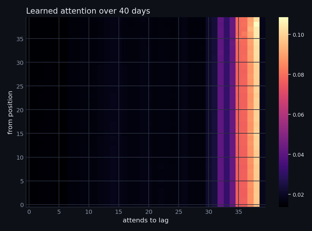
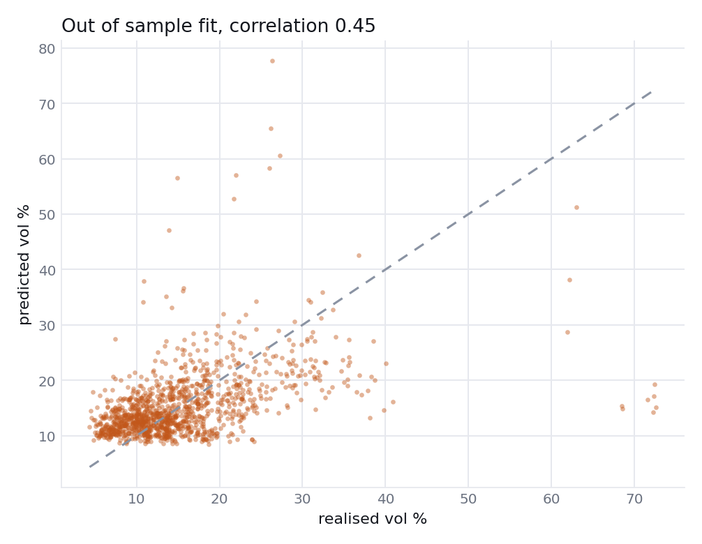
Result. Correlation 0.446 and a root mean squared error of 7.81 volatility points, against 0.457 and 7.74 for the LSTM on identical data. Read alone that looks like a loss for attention. Read against five seeds of each, in section 6, the gap sits inside the noise on four seeds out of five, so the honest call is that neither separates on a sequence this short and the transformer is the less stable of the two. Forty numbers in a row give attention no long range dependency to exploit. Reach for it when the sequence is long or the dependencies genuinely skip.
Forty daily returns is a toy sequence, useful for showing the mechanism side by side with an LSTM on equal terms. Real money sits in language. Filings, earnings call transcripts, central bank statements and news wires arrive as text, in volumes no analyst can read, and transformers convert that stream into a number a model can trade on.
FinBERT is the standard entry point, from Araci (2019). BERT gets fine tuned on financial text, so it learns that "liability" is neutral accounting vocabulary rather than a complaint, and that "beat expectations" and "missed guidance" carry opposite signs even when the surrounding prose looks identical. Output is a sentiment score per sentence or per document, which then joins a signal alongside price and fundamental features. Typical uses: scoring the tone of an earnings call against the same company's previous calls, flagging changes in risk factor language between two 10-K filings, and building a news sentiment feed for a systematic equity book.
Nothing on this page runs FinBERT, and no sentiment result is claimed here. Section exists to put the volatility experiment in proportion: attention on a forty step return series is the small application, and reading a market's own words is the large one.
Autoencoders learn to copy their input, through a bottleneck too narrow to let everything pass. Encoder compresses, decoder rebuilds, and training minimises the difference between what went in and what came back. Nothing is labelled, so this is unsupervised work: whatever makes it through three units is the structure that 45 series genuinely share, and whatever gets lost is idiosyncratic.
Think of it as PCA that is allowed to bend. Linear PCA finds the eigenvectors of a covariance matrix; an autoencoder with nonlinear activations can find a curved manifold instead, which matters when correlations themselves change with the level of stress. Shape here follows Gu, Kelly and Xiu's conditional autoencoder work on latent asset pricing factors.
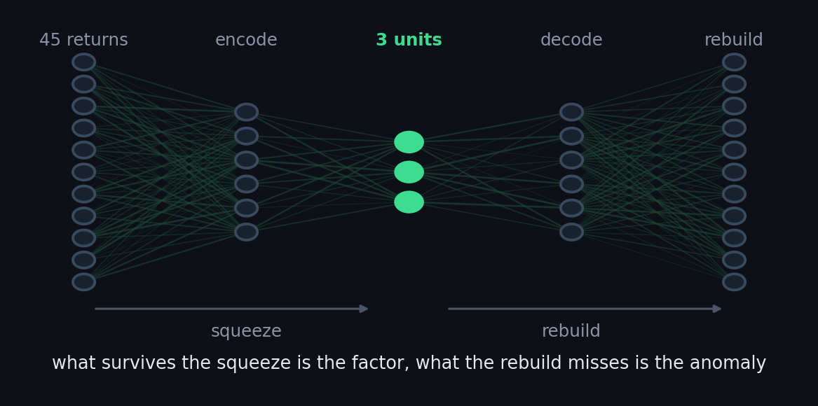
Statistical arbitrage lives on this. Strip the latent factors out of a return and what remains is a residual, and pairs and basket trades are bets that residuals mean revert. Risk teams use the same compression to build a factor covariance matrix that a portfolio optimiser can actually invert. Reconstruction error doubles as an anomaly detector, so a day the model cannot rebuild is a day the usual relationships stopped holding, which is a live input for regime and stress monitoring.
Universe spans ten sectors, from tech and banks through energy, staples and utilities, so the cross section being squeezed is more than several flavours of the same trade. Returns are standardised using training period statistics only, clipped at eight standard deviations, and the split is again by date at 75%.
Encoder to three units, decoder back to forty five
R = close.pct_change().dropna()
mu, sd = R.iloc[:int(len(R) * .75)].mean(), R.iloc[:int(len(R) * .75)].std()   # TRAIN stats only
Z = ((R - mu) / sd).clip(-8, 8).values.astype(np.float32)
n, cut = Z.shape[1], int(len(Z) * .75)

class AE(nn.Module):
    def __init__(self, n, k=3):
        super().__init__()
        self.enc = nn.Sequential(nn.Linear(n, 24), nn.Tanh(), nn.Linear(24, k))
        self.dec = nn.Sequential(nn.Linear(k, 24), nn.Tanh(), nn.Linear(24, n))
    def forward(self, x):
        z = self.enc(x)
        return self.dec(z), z

ae = AE(n).to(DEV); opt = torch.optim.Adam(ae.parameters(), lr=2e-3, weight_decay=1e-5)
for ep in range(400):
    idx = np.random.permutation(cut)[:1024]
    opt.zero_grad()
    rec, _ = ae(zt[idx].to(DEV))
    F.mse_loss(rec, zt[idx].to(DEV)).backward()
    opt.step()

erro = ((Z - rec) ** 2).mean(1)                       # per day reconstruction error
r2   = 1 - erro[cut:].mean() / (Z[cut:] ** 2).mean()  # 0.350 out of sample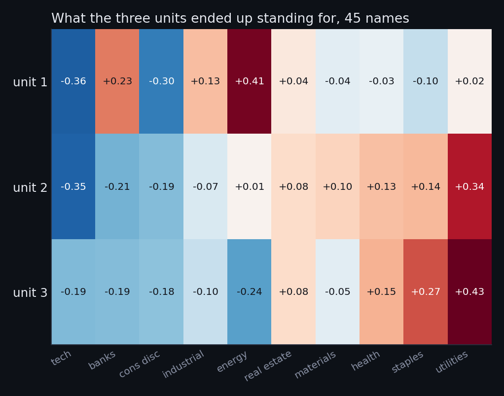
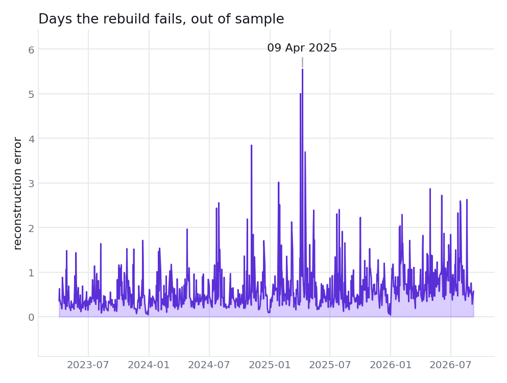
Result. 45 names over 3,440 days, out of sample from 4 April 2023, 35.0% of out of sample variance captured by three units, and a worst day of 9 April 2025. Three numbers standing in for 45 series, recovered without a single label.
Every number above was scored on its own. That answers "did it learn" and leaves open the question that matters on a desk, which is whether a model that costs nothing would have done as well. Three checks below, each run on the identical windows, rows and date split the networks were scored on, so nothing in the comparison comes from a different sample.
Three baselines for the ten day forward realised volatility target of sections 2 and 4. Persistence takes the realised vol of the last ten days and predicts it will continue. EWMA is the RiskMetrics filter with decay 0.94. HAR-RV, from Corsi (2009), regresses forward vol on daily, weekly and monthly realised vol, four coefficients fitted by least squares on the training block and frozen. Out of sample correlation with realised vol: persistence 0.49, EWMA 0.49, HAR-RV 0.53.
HAR-RV, the whole model
r2 = r ** 2                                            # squared daily log returns
rv1  = np.sqrt(r2) * np.sqrt(252)                      # today
rv5  = np.sqrt(r2.rolling(5).mean()) * np.sqrt(252)    # last week
rv22 = np.sqrt(r2.rolling(22).mean()) * np.sqrt(252)   # last month

A = np.c_[np.ones(len(rv1)), rv1, rv5, rv22]
beta, *_ = np.linalg.lstsq(A[:cut], fwd_vol[:cut], rcond=None)   # training block only
har = A[cut:] @ beta                                              # out of sample
Both networks were then retrained five times each from different seeds, nothing else changed. LSTM: 0.445, 0.464, 0.464, 0.488, 0.446. Transformer: 0.445, 0.451, 0.449, 0.384, 0.440. Means of 0.46 and 0.43, against 0.457 and 0.446 in the single published run.
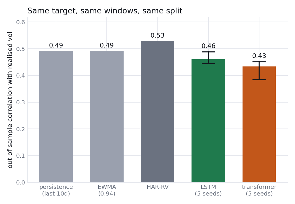
Reading is uncomfortable and clear. Ten day volatility on SPY is forecastable, and on forty daily absolute returns a linear model with the right three features extracts more of it than a recurrent cell or an attention head, at a small fraction of the cost. Nothing about that is a surprise to anyone who has run HAR on index vol; it is the reason HAR is the standard benchmark. Sections 2 and 4 stand as demonstrations of how each architecture reads a sequence. As forecasts, they lose to the boring thing, and the page should say so.
Seed by seed, LSTM minus transformer: 0.000, 0.013, 0.015, 0.104, 0.006. Three of the five gaps sit inside 0.015, one is zero, and the mean of 0.028 is carried almost entirely by a single transformer seed that collapsed to 0.38. A fair verdict on a sequence this short is that neither architecture separates from the other, and the transformer is the less stable of the two. Earlier versions of section 4 called it a loss for attention; the seeds do not support a call that strong.
Section 3 rescales prices inside each window so that only shape survives. That is the design of the original paper, and it is the right design for a direction question. For a magnitude question it throws away the single most useful number, which is how much the name moved over those same twenty days. Scoring that number on the identical 38,250 out of sample rows gives correlation 0.51 with forward vol, against 0.23 for the network. Quintile ladders, quietest to wildest: trailing vol 18 / 22 / 25 / 28 / 36, network 23 / 24 / 25 / 27 / 31.
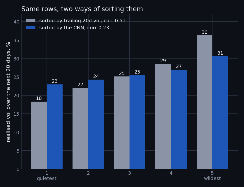
Verdict for section 3 changes accordingly. Shape carries roughly a quarter of the volatility information that level carries. A convolutional net on a scale free image is the wrong tool for a magnitude question and the right tool for the direction question the paper asked, where the direction result on 45 names came back as noise. Both findings point the same way: on this universe, price pictures did not earn their cost.
Two verdicts survive untouched. Feed forward on the surface has no baseline here because the option chain is only quoted during market hours and the comparison, a spline or SVI per expiry, is queued. Autoencoder factors have no obvious linear competitor beyond PCA, and the sector structure it recovered is visible in the loadings themselves.
Everything above reproduces from two scripts and free data. What follows is what is still wrong with it, because a results page without this section is asking to be believed rather than checked.
auto_adjust=True applies today's
split and dividend factors across the whole history, so a 2013 price reflects decisions made
later. Standard practice, and still not strictly point in time.
None of this makes the exercise pointless. It makes it a set of worked examples, each showing which architecture suits which shape of data, with the failure kept in view alongside the successes.
| Architecture | Task | Result | Against | Verdict |
|---|---|---|---|---|
| Feed forward | SPY implied vol surface | RMSE 0.251 vol pts | quotes spanning 10 to 55 | Inside the spread |
| LSTM | 10 day forward realised vol | corr 0.457 | HAR-RV 0.528 on the same rows | Loses to a linear model |
| CNN, direction | Up or down over 20 days | 0.01 pp quintile spread | 0.18, 0.19, 0.16 on reruns | Coin flip |
| CNN, magnitude | 20 day realised vol from an image | corr 0.225, 22.9% to 30.6% | trailing vol 0.513 on the same rows | Shape carries a quarter of what level does |
| Transformer | Same target as the LSTM | corr 0.446 | 0.434 mean over 5 seeds, LSTM 0.461 | No separation, less stable |
| Autoencoder | Cross section of 45 names | 35.0% in 3 units | 45 raw series | Compresses, and dates the stress |
| HAR-RV, baseline | 10 day forward realised vol | corr 0.528 | four coefficients | Beats both networks |
| Trailing vol, baseline | 20 day realised vol, next 20 | corr 0.513, 18% to 36% | one number per row | Beats the image |
Matching the architecture to the shape of the data is half the lesson. A static map got a feed forward net and landed inside the bid ask spread. A sequence with clustering got a recurrent cell and produced a forecast that reads well on its own. Attention, given the same short sequence, landed in the same place with more variance. Pictures answered a magnitude question weakly and refused a direction question, twice.
Other half of the lesson is section 6, and it costs more to learn. Volatility is forecastable, and on this data a four coefficient linear model forecasts it better than either network, while the single number the CNN was denied forecasts it better than the CNN. Deep learning earns its cost when the input carries structure a linear model cannot hold, a cross section, an order book, a filing. On forty daily numbers it did not, and any page that shows a network without the boring thing beside it is hiding the comparison that decides whether to use it.
Deep learning earns its place when the data has structure a table cannot hold: a smile across strikes, a sequence with memory, a picture, a cross section with hidden factors. Point it at a flat table of engineered features and a gradient boosted tree usually wins, which is what the previous page found on a stock panel.