
Straddles and calendars priced off the SPY chain, Heston calibrated to 307 quotes, GJR-GARCH on twenty years of returns, a neural network that hedges an option, and the VIX futures basis trade. Free data throughout, and every model set against something simpler that it has to beat.
Volatility is the one input an option price doesn't show. Every model below attacks it from a different side: a trade that buys or sells it, a model that bends it across strikes, a forecast of where it goes next, a network that hedges against it, and a strategy that harvests the premium buyers pay for it.
Data comes from the Cboe delayed quotes feed and from yfinance. No API key, no
subscription, no vendor terminal. GARCH runs on the arch package and the hedging
network on PyTorch, on a GPU when there's one and on the CPU when there isn't.
Read the limitations before quoting any number here. Option numbers are one closing snapshot, the hedging network trains on simulated paths, and the early years of the VIX index are a reconstruction.
TradingAgents, the open source multi agent framework behind the paper that reports a Sharpe ratio of 8.21, running on DeepSeek. Installation from a clean folder, a full run from the command line, a desk that shows every agent's turn as it happens, and the final decision sent as an order to Interactive Brokers. Along the way, Microsoft run twice two minutes apart, same date and same models, comes back Overweight and then Underweight. Write up on Glassbench.
I post the models as I build them, the changes I make to them, and the results that did not work. Shorter than these write ups, and there are a lot more of them.
Follow me on X


Sections below walk through each model step by step, with the reasoning, the charts and the code that produces every number on the page. Each block runs as pasted, on free data.
A straddle buys the call and the put on one strike. Long, it pays when the stock runs far in either direction, and every quiet day costs a little of the premium. Short is the mirror image: keep the premium, pay for any big move. Price of a straddle is therefore the market's own estimate of how far the stock will travel before expiry, in dollars.
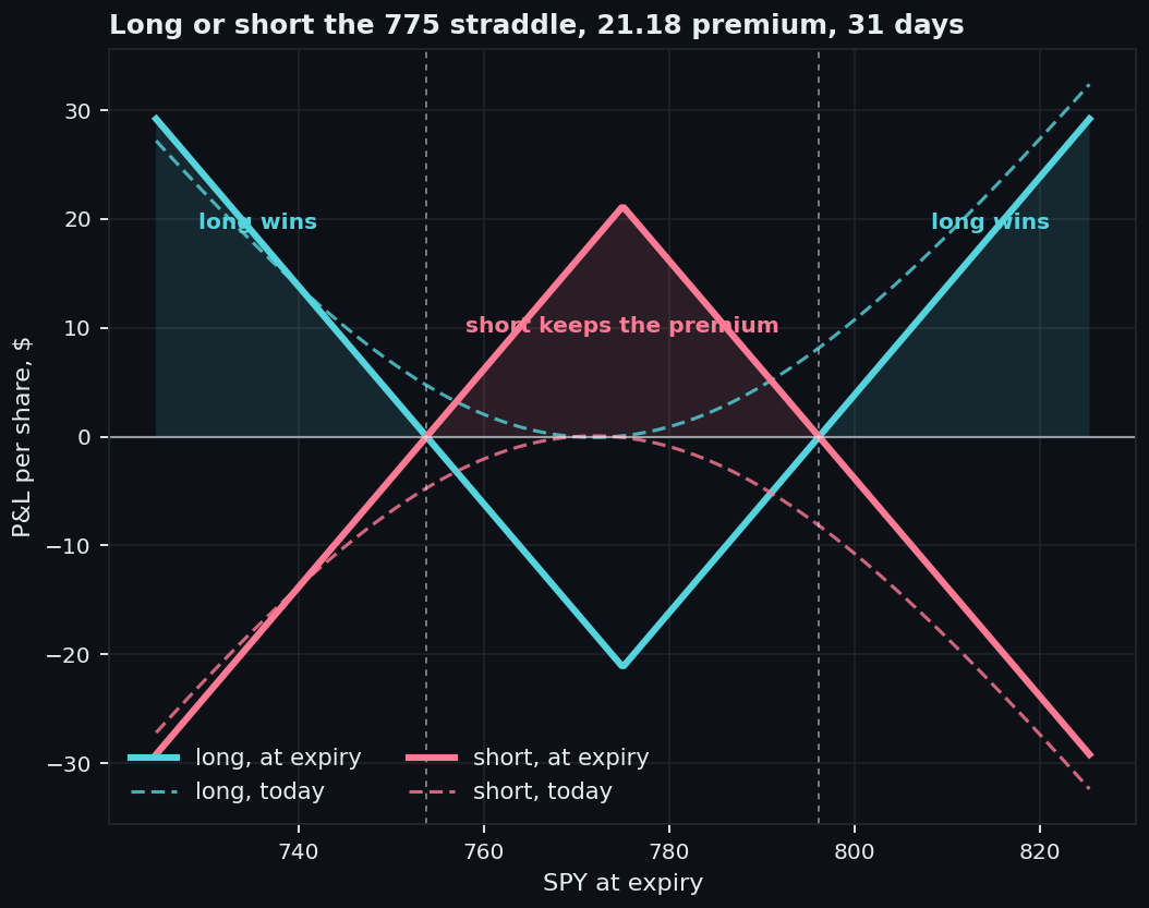
Volatility trading and event driven desks buy straddles into earnings and central bank days, when a jump is expected and its direction isn't. Option income funds and systematic premium sellers sit on the short side, collecting the premium the rest of the market pays for protection. A delta hedged straddle is a pure bet on realised against implied volatility: each day it earns half its gamma, times the stock price squared, times the gap between the realised and the implied variance, and loses when that gap is negative.
Quotes come from the Cboe delayed feed at the 22 September close, mid of bid and ask. SPY options are American, and early exercise on deep puts bends put call parity, so a regression of calls minus puts on strike gives a discount factor above one. Discount comes from the T-bill instead, and parity is used only for the forward, where the dividend shows up.
Cboe chain, forward from parity, Black 76 implied vol
import numpy as np, pandas as pd, requests
from scipy.stats import norm

# Cboe delayed quotes: every SPY option with bid, ask and last trade, no key needed
url = "https://cdn.cboe.com/api/global/delayed_quotes/options/SPY.json"
raw = requests.get(url, headers={"User-Agent": "Mozilla/5.0"}, timeout=60).json()["data"]
spot = float(raw["close"])

rows = []
for o in raw["options"]:
    s = o["option"]                                    # e.g. SPY261023C00775000
    rows.append(dict(expiry=pd.Timestamp("20" + s[3:9]), kind=s[9],
                     strike=int(s[10:]) / 1000, bid=o["bid"], ask=o["ask"],
                     last=o.get("last_trade_time")))
chain = pd.DataFrame(rows)
chain["mid"] = (chain.bid + chain.ask) / 2
asof = pd.to_datetime(chain["last"].dropna()).max().normalize()
chain["T"] = (chain.expiry - asof).dt.days / 365
r = 0.040                                              # 13 week T-bill, ^IRX

def forward(expiry):
    """SPY options are American, so parity only gives the forward, never the discount."""
    g = chain[chain.expiry == expiry]
    T = g["T"].iloc[0]; D = np.exp(-r * T)
    c, p = (g[g.kind == k].set_index("strike") for k in ("C", "P"))
    ks = c.index.intersection(p.index)
    ks = ks[abs(ks / spot - 1) < 0.02]
    return float(np.median(ks.values + (c.loc[ks, "mid"].values - p.loc[ks, "mid"].values) / D)), D, T

def black(F, K, T, D, vol, call=True):
    d1 = (np.log(F / K) + vol * vol * T / 2) / (vol * np.sqrt(T)); d2 = d1 - vol * np.sqrt(T)
    if call:
        return D * (F * norm.cdf(d1) - K * norm.cdf(d2))
    return D * (K * norm.cdf(-d2) - F * norm.cdf(-d1))

def implied_vol(price, F, K, T, D, call=True):
    lo, hi = 1e-4, 3.0
    for _ in range(60):                                # bisection, error below 1e-15
        mid = (lo + hi) / 2
        lo, hi = (lo, mid) if black(F, K, T, D, mid, call) > price else (mid, hi)
    return (lo + hi) / 2
Straddle, implied move, and the calendar at the front expiry
def mid(expiry, kind, K):
    return chain.query("expiry == @expiry and kind == @kind and strike == @K").mid.iloc[0]

front = chain.loc[(chain["T"] * 365 - 30).abs().idxmin(), "expiry"]   # 23 Oct, 31 days
back = chain.loc[(chain["T"] * 365 - 59).abs().idxmin(), "expiry"]    # 20 Nov, 59 days
K = 775.0                                              # strike listed on both expiries

straddle = mid(front, "C", K) + mid(front, "P", K)
print(f"straddle {straddle:.2f}, implied move {straddle / spot:.2%}")
print(f"breakevens {K - straddle:.2f} and {K + straddle:.2f}")

Ff, Df, Tf = forward(front); Fb, Db, Tb = forward(back)
iv_front = implied_vol(mid(front, "C", K), Ff, K, Tf, Df)
iv_back = implied_vol(mid(back, "C", K), Fb, K, Tb, Db)
calendar = mid(back, "C", K) - mid(front, "C", K)

# value of the calendar on the day the front month expires, across spot
spot_grid = np.linspace(0.92 * K, 1.08 * K, 400)
left = Tb - Tf
back_value = black(spot_grid * np.exp(r * left), K, left, np.exp(-r * left), iv_back)
pnl = back_value - np.maximum(spot_grid - K, 0) - calendar
print(f"calendar {calendar:.2f}, best case {pnl.max():.2f}")
print(f"profitable between {spot_grid[pnl > 0].min():.0f} and {spot_grid[pnl > 0].max():.0f}")| Trade | Legs | Cost | Reading |
|---|---|---|---|
| Straddle | +call +put 775, 31d | 21.18 | implied move 2.74% |
| Breakevens | at expiry | 753.83 and 796.17 | |
| Calendar | -call 31d, +call 59d | 7.37 | best case +5.25 |
| Calendar range | profitable at front expiry | 764 to 789 | |
| Implied vol | front / back | 11.76% / 13.41% |
A 2.7% move priced over a month is calm for SPY, and the front implied vol of 11.8% says the same. Calendar costs 7.37 and makes at most 5.25, only if SPY sits right on 775 on the first expiry, which is the price of owning time decay: a narrow window of profit and a wide one of small losses.
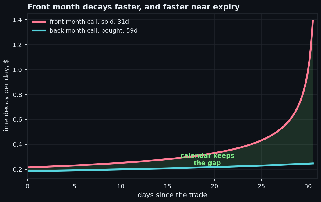
Both legs lose value every day, the one sold faster than the one bought. Near dated time decay is small at first and explodes in the last week, while a two month option barely notices the same days. Calendar keeps the gap, and the gap is widest right before the front expiry.
Time decay of each leg as the days pass
def theta_per_day(K, T, vol):
    d1 = (vol * vol * T / 2 + r * T) / (vol * np.sqrt(T)); d2 = d1 - vol * np.sqrt(T)
    return (-K * norm.pdf(d1) * vol / (2 * np.sqrt(T))
            - r * K * np.exp(-r * T) * norm.cdf(d2)) / 365

for days_gone in (0, 15, 25, 30):
    f = -theta_per_day(K, Tf - days_gone / 365, iv_front)
    b = -theta_per_day(K, Tb - days_gone / 365, iv_back)
    print(f"day {days_gone:2d}: front loses {f:.2f}, back loses {b:.2f}, calendar keeps {f - b:.2f}")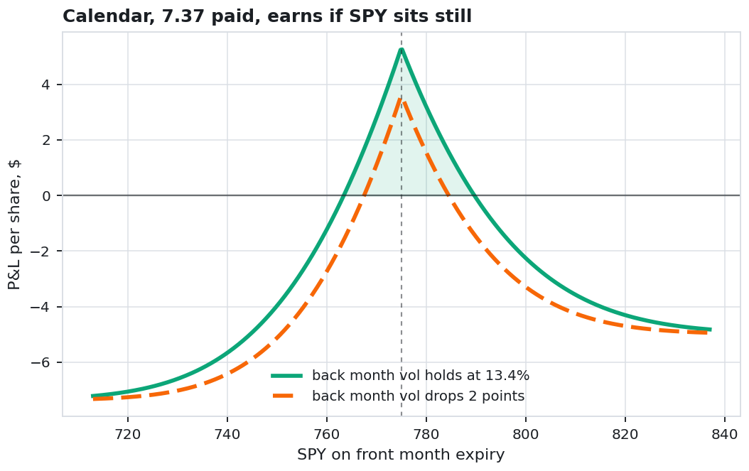
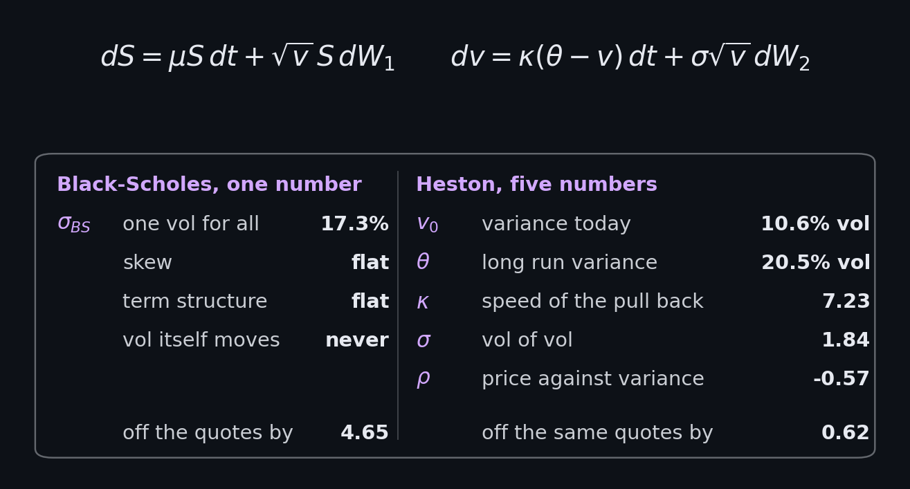
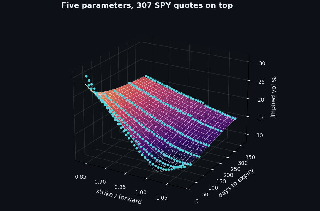
Black-Scholes gives one volatility for every strike and every expiry, and the market quotes a different one for each. Heston lets variance follow its own random process, pulled back to a long run level, with its shocks correlated to price. Negative correlation is what makes low strikes expensive, and a variance that moves is what gives the surface its term structure.
Index option desks, exotics books and risk management calibrate some version of Heston every morning. It prices path dependent products consistently with the vanilla surface, gives a hedge ratio that knows vol moves with spot, and its characteristic function makes pricing a whole chain take milliseconds. Stochastic local vol models used on exotic desks start from it.
No simulation is needed for vanillas. Characteristic function of the log price is known in closed form, and one integral turns it into a call price. Two numerical details decide whether the fit works: the branch of the complex logarithm, and fixed quadrature nodes, so the optimiser sees a smooth function instead of adaptive noise.
Heston characteristic function and Lewis pricing
def heston_cf(u, T, v0, kappa, theta, sigma, rho):
    """Characteristic function of log(S_T / F), Albrecher's branch (the little trap).
    The textbook branch crosses the log's branch cut at long maturities and returns
    prices outside the no arbitrage bounds."""
    xi = kappa - rho * sigma * 1j * u
    d = np.sqrt(xi ** 2 + sigma ** 2 * (1j * u + u ** 2))
    g = (xi - d) / (xi + d)
    e = np.exp(-d * T)
    C = kappa * theta / sigma ** 2 * ((xi - d) * T - 2 * np.log((1 - g * e) / (1 - g)))
    D = (xi - d) / sigma ** 2 * ((1 - e) / (1 - g * e))
    return np.exp(C + D * v0)

# fixed Gauss Legendre nodes on [0, 400]: the optimiser sees a smooth function
x, w = np.polynomial.legendre.leggauss(400)
U, W = 200 * (x + 1), 200 * w

def heston_call(F, K, T, disc, *p):
    """Lewis single integral, vectorised over every strike of one expiry."""
    k = np.log(K / F)
    phi = heston_cf(U - 0.5j, T, *p)
    integrand = (np.exp(-1j * np.outer(k, U)) * phi / (U ** 2 + 0.25)).real
    return disc * (F - np.sqrt(F * K) / np.pi * (integrand @ W))
Seven smiles from the same chain
def smile_quotes(expiry):
    """Out of the money only, strikes every $5 between 0.82 and 1.10 of the forward,
    bid above 5 cents and spread under a quarter of the mid."""
    F, D, T = forward(expiry)
    g = chain[chain.expiry == expiry].copy()
    g = g[((g.kind == "C") & (g.strike >= F)) | ((g.kind == "P") & (g.strike < F))]
    g = g[(g.bid > 0.05) & ((g.ask - g.bid) / g.mid < 0.25) & (g.strike % 5 == 0)
          & (g.strike / F > 0.82) & (g.strike / F < 1.10)]
    g["F"], g["D"] = F, D
    g["iv"] = [implied_vol(m, F, k, T, D, c == "C") for m, k, c in zip(g.mid, g.strike, g.kind)]
    return g[(g.iv > 0.03) & (g.iv < 1.0)]

days = chain.drop_duplicates("expiry").set_index("expiry")["T"] * 365
days = days[days >= 7]
picked = []
for target in (21, 45, 75, 120, 180, 270, 365):       # seven expiries, a month to a year
    left = days.drop(picked)
    picked.append((left - target).abs().idxmin())
q = pd.concat([smile_quotes(e) for e in picked], ignore_index=True)
print(f"{len(q)} quotes on {q.expiry.nunique()} expiries")
Calibration on vega weighted errors, and the one vol benchmark
from scipy.optimize import least_squares

d1 =(np.log(q.F / q.strike) + q.iv ** 2 * q["T"] / 2) / (q.iv * np.sqrt(q["T"]))
q["vega"] = q.D * q.F * norm.pdf(d1) * np.sqrt(q["T"])

def residuals(p):
    out = []
    for _, g in q.groupby("expiry"):
        F, D, T = g.F.iloc[0], g.D.iloc[0], g["T"].iloc[0]
        c = heston_call(F, g.strike.values, T, D, *p)
        model = np.where(g.kind == "C", c, c - D * (F - g.strike.values))
        out.append((model - g.mid.values) / g.vega.values)    # dollars to vol points
    return np.concatenate(out)

fit = least_squares(residuals, x0=[0.02, 2.0, 0.04, 0.8, -0.7], x_scale="jac",
                    bounds=([1e-4, 0.05, 1e-4, 0.05, -0.999], [0.5, 15, 0.5, 3, 0.5]))
v0, kappa, theta, sigma, rho = fit.x
print(f"vol today {np.sqrt(v0):.1%}, long run {np.sqrt(theta):.1%}, kappa {kappa:.2f}, "
      f"vol of vol {sigma:.2f}, rho {rho:.2f}, Feller {2 * kappa * theta > sigma ** 2}")

# Black-Scholes on the same ruler: the best single vol is the mean, its miss the std
print(f"one vol {q.iv.mean():.1%} misses by {100 * q.iv.std(ddof=0):.2f} vol points")| Parameter | Meaning | Value |
|---|---|---|
| v0 | variance today | 0.0112 (10.6% vol) |
| theta | long run variance | 0.0421 (20.5% vol) |
| kappa | speed of the pull back | 7.23 |
| sigma | vol of vol | 1.84 |
| rho | price against variance | -0.57 |
| Feller | 2 kappa theta above sigma squared | fails |
| Model | Free numbers | Fit error |
|---|---|---|
| Black-Scholes | 1 | 4.65 |
| Heston | 5 | 0.62 |
| Heston, 69 day smile only | 5 | 0.57 |
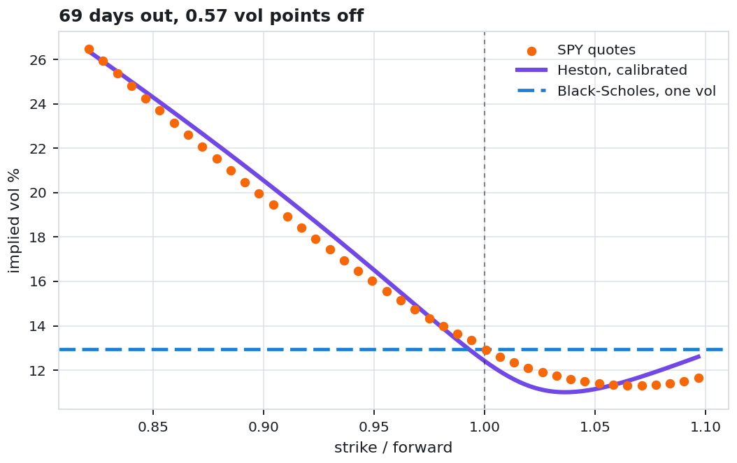
Best single vol across all 307 quotes is 17.3%, and it misses by 4.65 points, because the surface runs from the low teens at the money to the high twenties on the downside. Five Heston numbers bring the miss down to 0.62. Correlation lands at -0.57, vol of vol at 1.84, high enough to break the Feller condition, a common result on equity index data that lets variance touch zero.
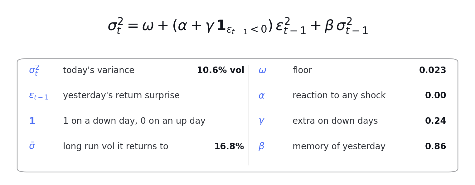
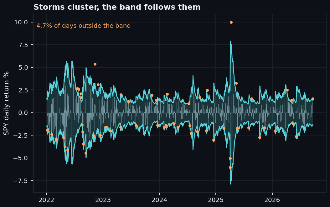
Volatility clusters: a violent day tends to follow a violent day. GARCH turns that into a recursion, where today's variance is a floor, plus a share of yesterday's squared surprise, plus a share of yesterday's variance. GJR adds one term that fires only on down days, and on SPY that term turns out to carry the whole effect.
Market risk teams run it daily for value at risk, portfolio construction uses it to scale position sizes to the volatility expected tomorrow, and options desks compare its forecast with implied vol to decide whether options look cheap or dear. It's cheap to fit, easy to explain to a risk committee, and still hard to beat at short horizons.
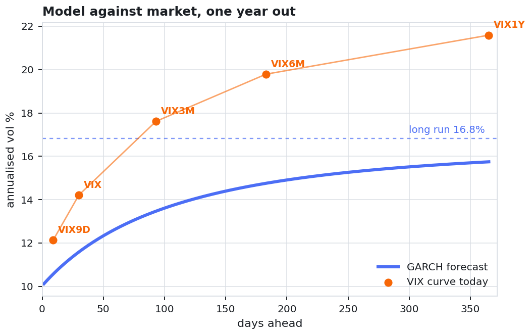
Plain GARCH with fat tails was fitted first and rejected: its persistence came out at 0.994, almost a unit root, and its long run volatility at 27.8% for an index that actually averaged 18.9% over the sample. Adding the GJR term improves the log likelihood by about 100 for one extra parameter and brings the long run level back to 16.8%.
GJR-GARCH with Student t errors, and the forecast curve
import numpy as np, pandas as pd, yfinance as yf
from arch import arch_model

spy = yf.download("SPY", start="2005-01-01", auto_adjust=True)["Close"].squeeze()
r = 100 * np.log(spy).diff().dropna()

# o=1 adds the GJR term: gamma fires only on down days. Student t for the fat tails.
res = arch_model(r, mean="Constant", vol="GARCH", p=1, o=1, q=1, dist="t").fit(disp="off")
a, g, b = res.params["alpha[1]"], res.params["gamma[1]"], res.params["beta[1]"]
lam = a + b + g / 2
print(f"alpha {a:.3f}, gamma {g:.3f}, beta {b:.3f}, persistence {lam:.3f}")
print(f"half life {np.log(0.5) / np.log(lam):.0f} days, "
      f"long run {np.sqrt(252 * res.params['omega'] / (1 - lam)):.1f}%")

# average vol expected over every horizon up to a year, to set against the VIX curve
var = res.forecast(horizon=252, reindex=False).variance.values[-1]
curve = np.sqrt(252 * np.cumsum(var) / np.arange(1, 253))| Parameter | Meaning | Value |
|---|---|---|
| omega | floor | 0.0227 |
| alpha | reaction to any shock | 0.000 |
| gamma | extra reaction on down days | 0.242 |
| beta | memory of yesterday's variance | 0.859 |
| nu | Student t degrees of freedom | 5.9 |
| persistence | alpha + beta + gamma / 2 | 0.980 |
| half life | days for a shock to fade by half | 34 |
| long run vol | where it returns | 16.8% |
| vol today | as of 2026-09-21 | 10.6% |
Alpha lands on zero and gamma at 0.24: an up day adds nothing to tomorrow's variance, a down day adds a quarter of its square. That asymmetry, the leverage effect, is exactly what makes put options on the index expensive, and it's the same story the Heston correlation of -0.57 tells from the option side.
Parameters are estimated on data up to 2019 only and then just filtered forward, so every forecast since 2020 uses nothing the model could not have known. Each day it forecasts the average vol of the next 21 trading days, and so does the VIX, in its own way.
Out of sample test from 2020, against realised vol and the VIX
# out of sample: parameters estimated ONLY on data to 2019, then filtered forward
p19 = arch_model(r[:"2019-12-31"], p=1, o=1, q=1, dist="t").fit(disp="off").params
s2 = arch_model(r, p=1, o=1, q=1, dist="t").fix(p19).conditional_volatility.values ** 2
lam19 = p19["alpha[1]"] + p19["beta[1]"] + p19["gamma[1]"] / 2
long_run = p19["omega"] / (1 - lam19)
eps = r.values - p19["mu"]
s2_next = p19["omega"] + (p19["alpha[1]"] + p19["gamma[1]"] * (eps < 0)) * eps ** 2 + p19["beta[1]"] * s2
decay = (lam19 ** np.arange(21)).mean()                # closed form, 21 day average
forecast = np.sqrt(252 * (long_run + decay * (s2_next - long_run)))
realised = np.sqrt(252 * pd.Series(r.values ** 2).rolling(21).mean().shift(-21).values)

vix = yf.download("^VIX", start="2005-01-01")["Close"].squeeze().reindex(r.index).values
d = pd.DataFrame(dict(garch=forecast, vix=vix, real=realised), index=r.index)["2020":].dropna()
print(d.corr()["real"].round(2))| Forecast | Correlation with realised |
|---|---|
| GJR-GARCH, fitted to 2019 | 0.59 |
| VIX | 0.56 |
A model with five numbers fitted before the pandemic tracks realised vol about as well as the VIX does, 0.59 against 0.56. VIX sat above the realised vol that followed on 85% of days, by 3.9 points on average. That gap is the variance risk premium, and section 5 is a strategy built to collect it.
Bühler, Gonon, Teichmann and Wood asked in 2019 whether a neural network can hedge an option with no pricing model at all, given only price paths and the real cost of trading. Each day the network sees moneyness, time left and the shares it already holds, and picks the new position. It's trained end to end through thirty days of trading, directly on the tail of the profit and loss.
Derivatives desks, market makers and structured products teams hedge books where every rebalance costs money and the textbook delta assumes it doesn't. A learned policy trades off hedging error against cost on its own, respects any risk measure written as a loss, and can be retrained overnight when the cost model or the market changes.
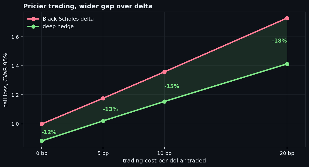
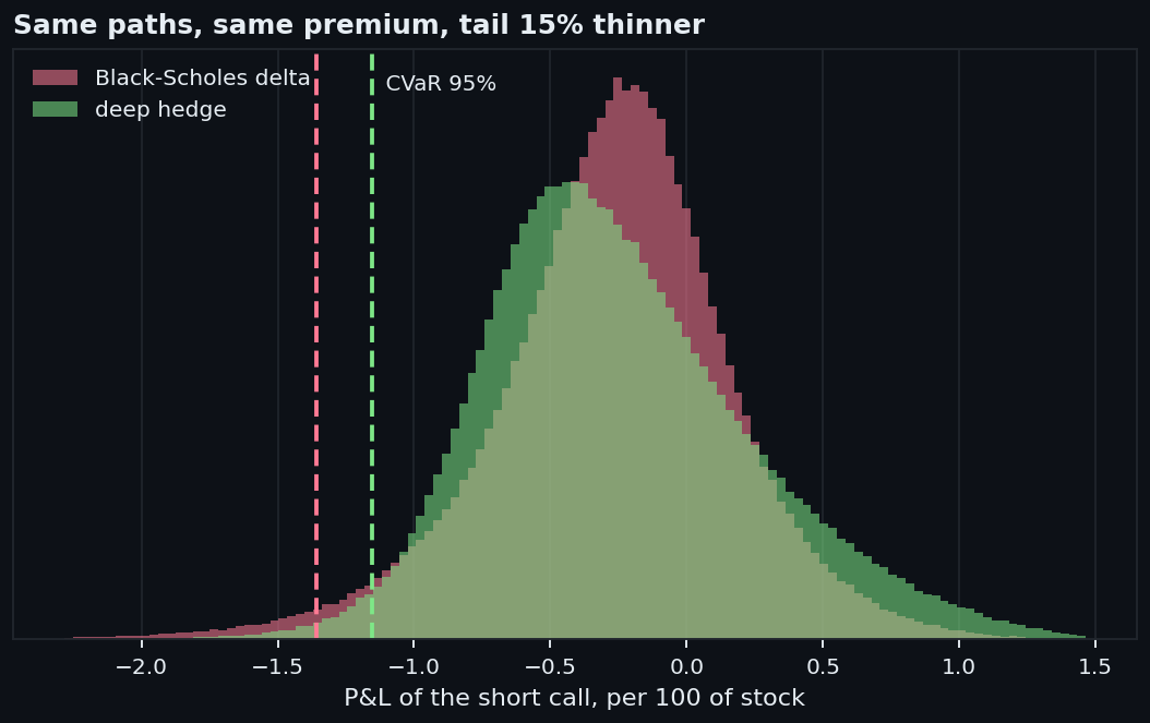
Sold: one 30 day at the money call, hedged once a day with the stock, 10 basis points charged on every dollar traded, including the unwind. Loss is CVaR at 95%, the average of the worst 5% of outcomes, written in the Rockafellar and Uryasev form so the threshold is learned alongside the network. Sixteen thousand fresh paths per step, three thousand steps.
Recurrent hedge, trading costs, and a CVaR objective
import math, numpy as np, torch, torch.nn as nn
DEV = "cuda" if torch.cuda.is_available() else "cpu"

S0 = K = 100.0; SIG = 0.20; N = 30; T = N / 252; DT = T / N
C = 0.001                                               # 10 bp on every dollar traded
d1 = (SIG * SIG * T / 2) / (SIG * math.sqrt(T))
PREMIUM = S0 * 0.5 * (1 + math.erf(d1 / 2 ** 0.5)) - K * 0.5 * (1 + math.erf((d1 - SIG * math.sqrt(T)) / 2 ** 0.5))
TAU = torch.tensor([T - k * DT for k in range(N)], device=DEV)

def paths(n):
    z = torch.randn(n, N, device=DEV)
    ls = math.log(S0) + torch.cumsum(-SIG ** 2 / 2 * DT + SIG * math.sqrt(DT) * z, 1)
    return torch.cat([torch.full((n, 1), S0, device=DEV), torch.exp(ls)], 1)

net = nn.Sequential(nn.Linear(3, 64), nn.SiLU(), nn.Linear(64, 64), nn.SiLU(),
                    nn.Linear(64, 1)).to(DEV)

def policy(t, S_t, held):
    m = torch.log(S_t / K) / (SIG * torch.sqrt(TAU[t]))
    x = torch.stack([m.clamp(-4, 4), (TAU[t] / T).expand_as(m), held], 1)
    return torch.sigmoid(net(x)).squeeze(1)             # a call delta lives in [0, 1]

def hedge_pnl(S, rule, c=C):
    """Seller of the call: premium in, hedge gains, trading costs, payoff out."""
    held = torch.zeros(S.shape[0], device=DEV)
    pnl = torch.full_like(held, PREMIUM)
    for t in range(N):
        new = rule(t, S[:, t], held)
        pnl += new * (S[:, t + 1] - S[:, t]) - c * S[:, t] * (new - held).abs()
        held = new
    return pnl - c * S[:, -1] * held - torch.clamp(S[:, -1] - K, min=0)

w = torch.zeros(1, device=DEV, requires_grad=True)     # the VaR, learned jointly
opt = torch.optim.Adam(list(net.parameters()) + [w], lr=2e-3)
sched = torch.optim.lr_scheduler.CosineAnnealingLR(opt, 3000)
for step in range(3000):
    pnl = hedge_pnl(paths(16384), policy)
    loss = w + torch.relu(-pnl - w).mean() / 0.05       # CVaR 95%, Rockafellar and Uryasev
    opt.zero_grad(); loss.backward(); opt.step(); sched.step()
Test on 500,000 new paths against Black-Scholes delta
def bs_delta(t, S_t, held):
    d = (torch.log(S_t / K) + SIG ** 2 / 2 * TAU[t]) / (SIG * torch.sqrt(TAU[t]))
    return 0.5 * (1 + torch.erf(d / 2 ** 0.5))

def cvar(loss, a=0.95):
    return loss[loss >= np.quantile(loss, a)].mean()

with torch.no_grad():
    S = paths(500_000)                                  # never seen in training
    net_pnl = hedge_pnl(S, policy).cpu().numpy()
    bs_pnl = hedge_pnl(S, bs_delta).cpu().numpy()
print(f"CVaR 95%: network {cvar(-net_pnl):.3f}, delta {cvar(-bs_pnl):.3f}")| Trading cost | CVaR 95%, network | CVaR 95%, delta | Tail change | Turnover, network | Turnover, delta |
|---|---|---|---|---|---|
| 0 bp | 0.882 | 0.999 | -12% | 2.58 | 2.71 |
| 5 bp | 1.020 | 1.176 | -13% | 2.51 | 2.71 |
| 10 bp | 1.154 | 1.358 | -15% | 2.46 | 2.71 |
| 20 bp | 1.413 | 1.729 | -18% | 2.35 | 2.71 |
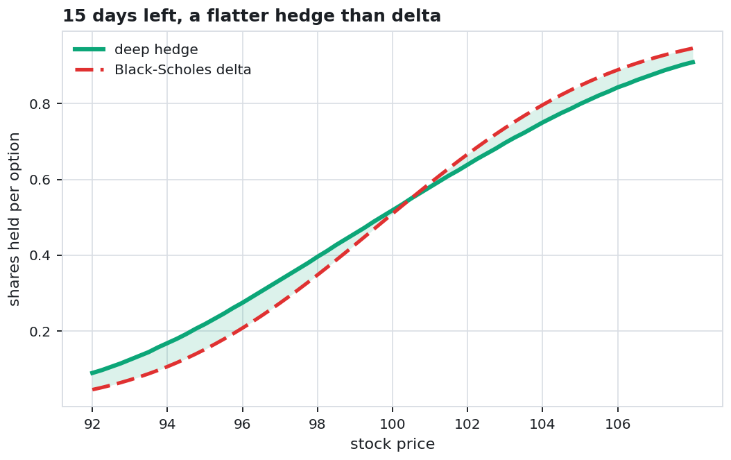
At 10 basis points the network cuts the tail by 15% and trades 10% less. Even at zero cost it still wins on the tail, because delta is only optimal when hedging never stops, and daily rebalancing leaves gaps that a policy aimed at the tail can use. What it learned is a flatter hedge than delta: more shares when the option is out of the money, fewer when it's in.
VIX futures usually trade above spot VIX. That contango is an insurance premium, and each future drifts down toward spot as it nears expiry, so a short position earns the roll. Simon and Campasano showed in 2014 that shorting the futures in contango and buying them in backwardation harvests it, and Quantpedia lists the rule among its best known volatility strategies. Short volatility ETFs are the retail version of the same trade.
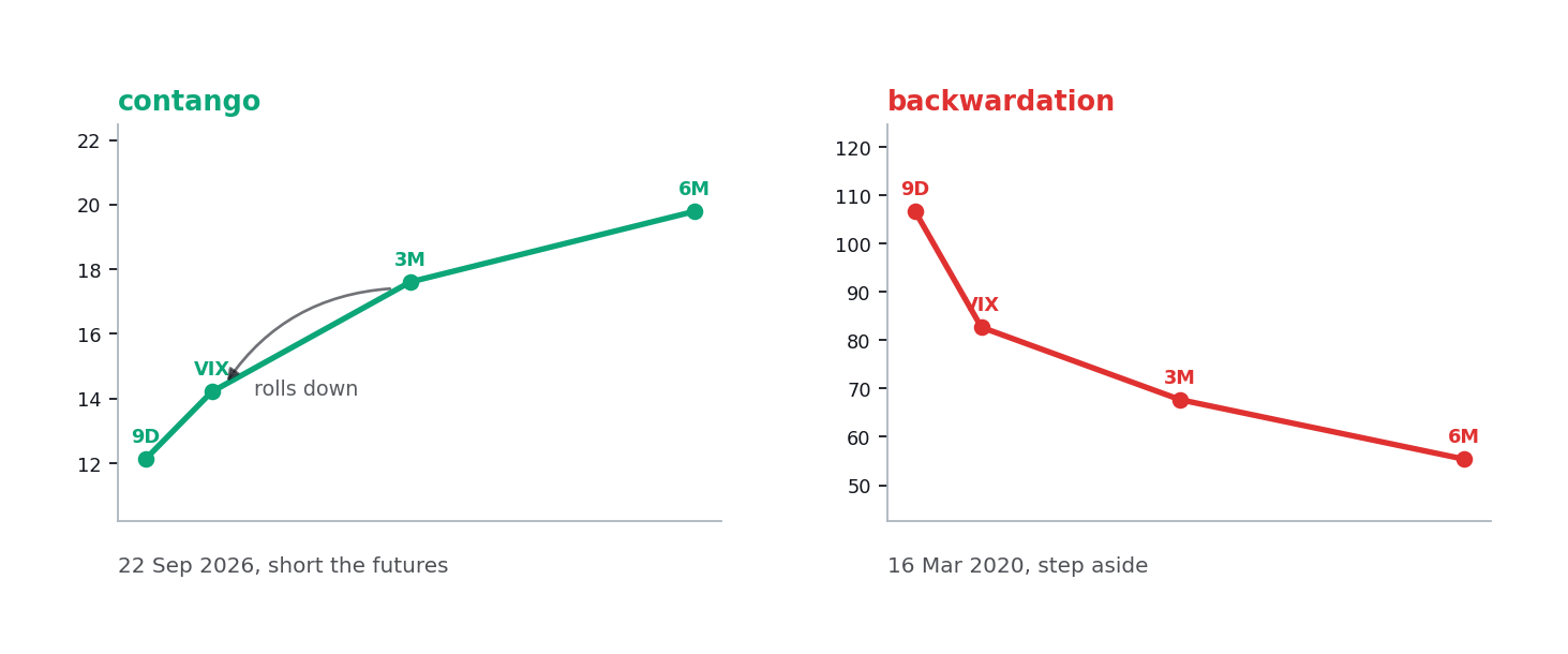
Volatility arbitrage funds and systematic premium sellers run versions of it, and tail hedging desks sit on the other side, paying the premium for protection. Volatility ETF issuers roll exactly these futures every day, which is part of why the roll is there to be collected.
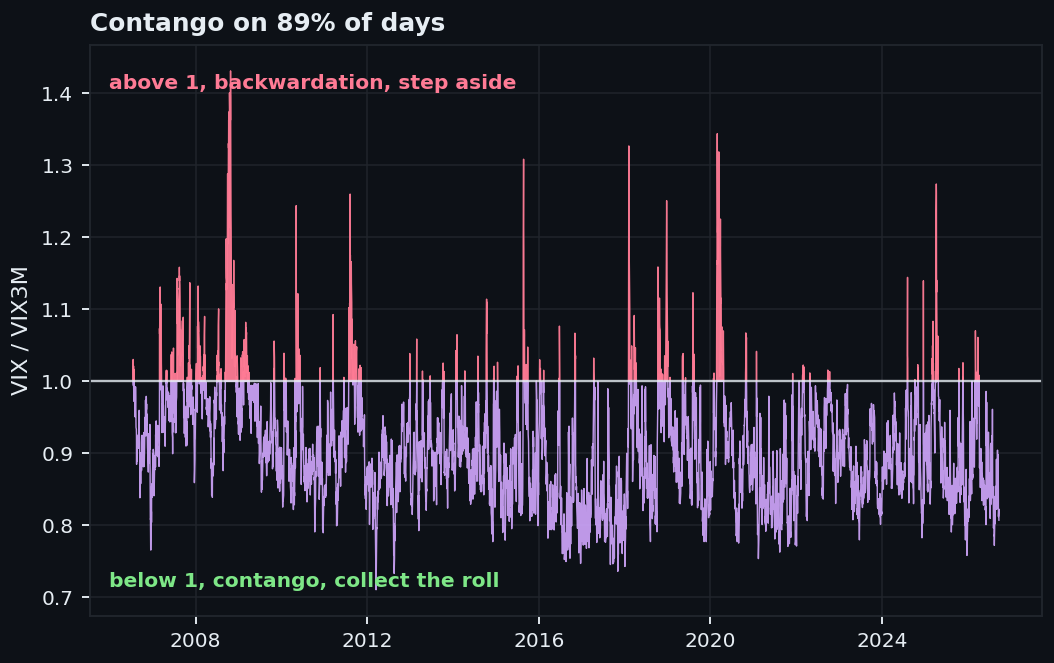
Returns come from the Cboe short VIX futures index, minus one times the daily move of the first and second month futures, the index the SVIX fund tracks. Signal is spot VIX against the three month VIX index, read at yesterday's close so the backtest never trades on information it didn't have. Every switch pays 10 basis points.
Signal, three rules, and their statistics
import numpy as np, pandas as pd, yfinance as yf

px = yf.download(["^VIX", "^VIX3M", "^SHORTVOL"], start="2006-07-17")["Close"].dropna()
ret = px["^SHORTVOL"].pct_change()                     # Cboe short VIX futures index

# decided at yesterday's close, applied to today's return
short = (px["^VIX"] < px["^VIX3M"]).astype(float).shift(1)
switch = short.diff().abs().fillna(0)
rules = pd.DataFrame({
    "always short": ret,
    "short in contango": short * ret - 0.001 * switch,
    "short contango, long backwardation": (2 * short - 1) * ret - 0.002 * switch,
}).dropna()

def stats(x):
    g = (1 + x).cumprod(); years = len(x) / 252
    return pd.Series({"CAGR %": 100 * (g.iloc[-1] ** (1 / years) - 1),
                      "vol %": 100 * x.std() * np.sqrt(252),
                      "Sharpe": x.mean() / x.std() * np.sqrt(252),
                      "max drawdown %": 100 * (g / g.cummax() - 1).min(),
                      "worst day %": 100 * x.min()})

print(rules.apply(stats).T.round(2))
print(f"contango on {(px['^VIX'] < px['^VIX3M']).mean():.0%} of days")
Tables below cover 2006-07-18 to 2026-09-22. Rerun the block on a later day and the figures move a little, since every new session enters a twenty year compounding.
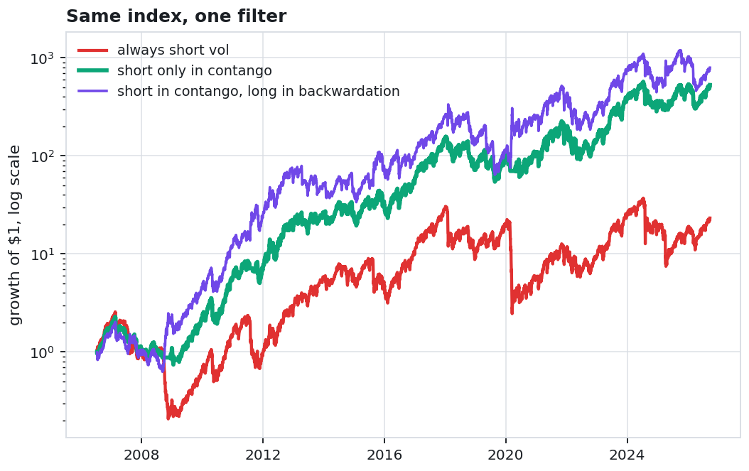
| Rule | CAGR | Volatility | Sharpe | Max drawdown | Worst day |
|---|---|---|---|---|---|
| Always short | 17.0% | 67.0% | 0.59 | -91.9% | -42.1% |
| Short only in contango | 36.7% | 56.2% | 0.85 | -67.6% | -30.1% |
| Short contango, long backwardation | 39.5% | 66.9% | 0.84 | -80.9% | -30.1% |
| Episode | Always short | Contango only | Long in backwardation |
|---|---|---|---|
| Autumn 2008 | -72.2% | 4.8% | 215.1% |
| February 2018 | -45.0% | -11.5% | 18.2% |
| March 2020 | -80.9% | -17.4% | 96.7% |
| August 2024 | -38.3% | -19.6% | -18.3% |
Always short compounded 17% a year and fell 92% from peak to trough. Stepping aside whenever VIX closes above VIX3M lifts that to 37% and cuts the worst drawdown to 68%, with the curve in contango on 89% of days and about 15 switches a year. Going long in backwardation, the full Simon and Campasano rule, makes a fortune in 2008 and 2020 and gives it back, with a deeper drawdown than the filter alone.
It still can't dodge the first day of a shock. On 12 June 2020 the filtered rule lost 30% in one session, because the curve was still in contango at the previous close. Any live version needs a position size that survives that day.
| Model | Task | Result | Against | Verdict |
|---|---|---|---|---|
| Straddle | price a 31 day move | 2.74% implied move | front vol 11.8% | Calm month priced |
| Calendar | own the time decay | 7.37 for up to +5.25 | profit 764 to 789 | Narrow window |
| Heston | fit 307 quotes | 0.62 vol pts | one BS vol 4.65 | Seven times tighter |
| GJR-GARCH | 21 day vol forecast | corr 0.59 | VIX 0.56 | Level with the VIX |
| Deep hedging | hedge a short call | tail -15% | Black-Scholes delta | Wins, simulated |
| VIX basis | 20 years of short vol | 37% a year, -68% DD | always short 17%, -92% DD | Filter pays |
Each model earns its place against something simpler, and each one fails somewhere the table can't show: the straddle on a day the move comes early, Heston on the far downside, GARCH on the first day of a shock, the hedging network on paths that don't look like its training set, and the VIX rule on a session like June 2020.