
Every model here is open source and every script below is runnable. Four of the six were executed while writing this page and their real output is printed underneath. What each model is for, the data it needs, and where it stops being free.
Volatility trading survives being wrong about direction. You are not betting the market goes up, you are betting the price of insurance is wrong. Which reduces the job to one number: what should that insurance cost.
That number comes from a model, and every model here is open source. Same families that price the book at a bank sit on GitHub. Models were never the expensive part. Data is.
Take six open source volatility models, work out what each actually does with the equations, then run all six on data that costs nothing.
Free data fights you. End of day files stamp a call and its put moments apart, so one strike can show its two legs disagreeing by 15 vol points. Wings are thin and their mids untrustworthy. History stops where it stops. Each bends a result, and each is named where it bites.
It still gets you further than expected. Free chains track VIX at 0.983. Heston calibrates to a real surface and returns a minus 0.54 skew nobody put there. A variance premium of 1.62 points falls out, positive two days in three, matching published work. Paid data buys precision and recency, not the mechanism.
These two cover the strategy side of volatility. This page is the toolbox underneath them.


They are not competitors. Several of them answer different questions about the same option, and you will end up using more than one. Ordered by how much they will actually change what you do, so start at the top. What separates them is what each one needs before it will produce a number.
| Tool | What it answers | Data it needs | Source |
|---|---|---|---|
| 1. SVI | one smooth smile through messy quotes | a real option chain | arXiv 1204.0646 |
| 2. arch | how volatile will it be next month, from prices alone | a return series, nothing else | bashtage/arch |
| 3. tf-quant-finance | the same price, hundreds of thousands at once | you supply the inputs | google/tf-quant-finance |
| 4. QuantLib | why the smile has the shape it does | a real chain to calibrate to, plus curves | lballabio/QuantLib |
| 5. FinancePy | implied vol back out of a price, and every greek | a real chain, the forward comes from it | domokane/FinancePy |
| 6. gs-quant | how a desk frames a vol screen | free prices, 46 of 48 functions need no credentials | goldmansachs/gs-quant |
A word about the data, because it is the honest limit of this page. The scripts run on free sources, Yahoo through yfinance and the free option chains from the data sources write up. That is enough to learn every one of these models properly and to feel how they behave. It is not what you would trade on. Free end of day quotes are stale, thin in the wings and occasionally wrong, and a model fed bad quotes will fit the noise with complete confidence. Treat this as a sandbox, and if a result starts to matter, pay for the data before you trust it.
Every model below is free. What decides whether the answer is any good is the chain you feed it, and that is where the money goes. So it is worth being precise about what this page runs on, and about what it would take to do the same work properly.
Free option data exists and it is better than people assume. What you can have for nothing is end of day quotes, on a handful of liquid underlyings, with history that stops a year or two back. That is genuinely enough to learn every model here, to see the shapes, and to test whether an idea is worth pursuing.
What you cannot have for free is the stuff that makes a number tradeable: a consistent snapshot time, the full strike grid including the illiquid wings, real forwards and dividends, and the last two years. Those are the four things you are actually buying, and none of them sound exciting until a result depends on them.
| Source | What it gave | Used for | Cost |
|---|---|---|---|
| Kaggle SPY chains | end of day chains with IV and greeks precomputed, 2016 to 2023, 8 of the 14 year files | every implied vol number here: the premium series, the SVI fit, the term structure | free, account and API token |
| yfinance | adjusted SPY daily closes | the GARCH fit and the realised volatility | free, no account |
| Kaggle SPX chains | SPX index chains in the same OptionsDX layout, 903 trading days, 191 strikes and 15 expiries a day | the SPX against SPY test below | free, account and API token |
| Cboe delayed quotes | a full live SPX or SPY chain as JSON, with IV and all five greeks, no account | the thin chain experiment in the SVI section, and the SPX forward check | free, one URL, no key |
| Cboe | the full VIX series from the exchange | checking the implied series was sane, see below | free, one CSV URL |
| Kaggle SPY chains | the 15 June 2023 chain, 8 expiries and 82 strikes at 29 days | the Heston calibration and the FinancePy inversion | free, account and API token |
| none | grid parameters chosen by hand | tf-quant-finance benchmark sizes only | not applicable |
All four are covered properly in the data sources write up, including which years and tickers each one reaches.
An honest list. Every row is a limit that was worked around rather than solved, and each one bends a result in a nameable direction.
| What is missing | Why it matters here | Where it comes from |
|---|---|---|
| the whole strike strip, not one strike | this is the largest single gap. Our at the money series sits 3.41 vol points under VIX, because VIX integrates the expensive downside puts and we read one strike. It makes the premium here understated | any full chain vendor, or compute it yourself from a complete grid |
| a consistent snapshot time | free end of day files stamp the two legs moments apart, which is how you get a call and a put at the same strike disagreeing by 15 vol points on a fast day | Cboe DataShop, ORATS, Polygon and similar, priced per dataset or per month |
| bid and ask, weighted | the fits here use unweighted mid IVs. Wings carry the widest spreads and the least trustworthy mids, so they should count for less. QuantLib below shows why this bites: calibration minimises error in price, which already tilts the fit toward the money before any weighting | already present in the Kaggle set and in the Cboe feed. It is the weighting step that is missing, not the data |
| the last two years | the Kaggle set stops at 2023, so nothing on this page says anything about 2024 onward | a live vendor subscription, or start snapshotting today |
Cheapest of those fixes is the last one, and it costs nothing but time. Options history is the one dataset you cannot buy back cheaply, so a cron job that snapshots the chains you care about tonight is worth more in a year than any single purchase you could make today.
Everything else sits on a ladder. Retail feeds like ORATS or Polygon get you consistent timestamps and a full grid for a monthly fee, which is the step that turns this from teaching into testing. OptionMetrics through WRDS is what the literature runs on and is priced for institutions. No prices are quoted here, because vendor pricing changes faster than this page will.
Worth showing, because it is the step people skip. That at the money implied series built from the Kaggle files correlates 0.983 with the VIX over the same 2016 to 2023 window, which says the series tracks reality. It also sits 3.41 points below it, which is not an error but the skew, and is exactly why the missing-strip row above is the one that matters most.
That same check catches real problems. Here is the February 2018 week read straight out of the 2018 file, next to what VIX did.
At the money implied vol by expiry, three days across the February 2018 volatility shock.
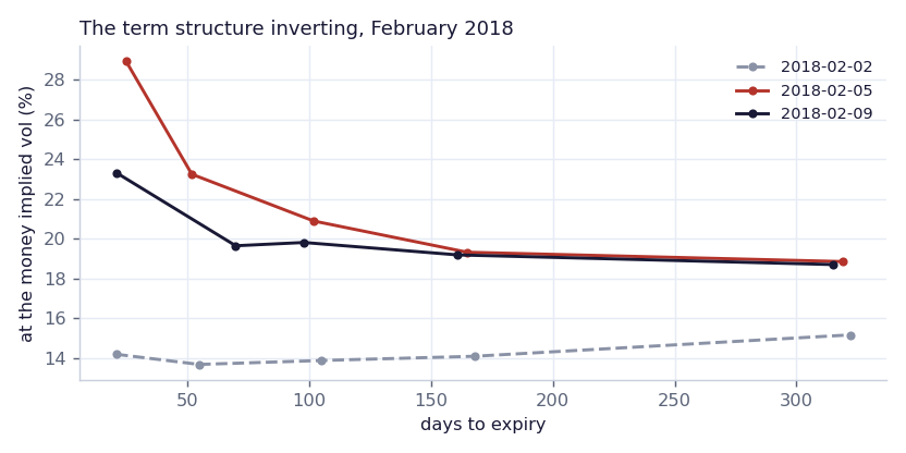
| Date | Our front month | VIX close |
|---|---|---|
| 2 February 2018 | 14.2% | 17.31 |
| 5 February 2018 | 28.9% | 37.32 |
| 9 February 2018 | 23.3% | 29.06 |
Everything on this page runs on SPY, an ETF: American style, pays dividends. Published work on the variance premium uses SPX, which is European and cash settled. Whether that substitution matters is testable rather than arguable, because free SPX chains exist for 2010 to 2013 and the SPY files cover the same years.
One caution about the SPX source. Its Kaggle listing is titled 2010 to 2023 and it is not. It stops on 16 August 2013, at 1,048,531 rows, and Excel's row ceiling is 1,048,576. Somebody opened it, it truncated silently, and that is what got uploaded. Worth checking the range of any file before trusting its title.
# pip install kagglehub pandas numpy yfinance
# the forward each strike implies, from put call parity: C - P = e^(-rT)(F - K)
w = d[(abs(np.log(d.STRIKE / spot)) < 0.03) & (d.C_BID > 0) & (d.P_BID > 0)].copy()
w["F_k"] = w.STRIKE + (w.cmid - w.pmid) / np.exp(-r * T)
F = float(w.F_k.median())
q = r - np.log(F / spot) / T          # the implied yield. on SPX this IS the dividend

# note the difference q_SPY - q_SPX is independent of r, since r cancels. so the
# comparison below does not depend on getting the rate right, only on using the same one.| Index | Median | IQR | Negative on | By year |
|---|---|---|---|---|
| SPX | 1.99% | 0.91 pts | 0.8% of days | 2.04, 1.95, 2.05, 1.75 |
| SPY | 0.45% | 4.50 pts | 31.9% of days | 1.10, 2.19, 2.31, -0.13 |
SPX lands on the real S&P dividend yield and stays there. SPY does not: it is 2.8 times more dispersed and returns a negative dividend yield on nearly a third of days, which is not a dividend at all but the early exercise value and borrow cost with nowhere else to go.
So the honest reading is that it depends entirely on which number is wanted:
| Quantity | Verdict |
|---|---|
| the forward, and any dividend backed out of the chain | badly distorted on SPY. Use SPX, or recover the forward and treat the yield as a plug rather than a forecast |
| at the money implied volatility | essentially identical. Correlation 0.9972 across 434 common days, SPX running 0.19 vol points lower |
| the variance risk premium | safe. SPX +1.76 mean and +1.96 median, positive 70.2% of days. SPY +1.88 and +2.20, positive 71.9% |
| Heston parameters | regime dependent, not index dependent. SPX June 2012 fits rho -0.7762 against SPY June 2023 at -0.5418, and the pricing error is 10.50% versus 10.29%. Nearly the same error on a different index in a different decade, which says the five parameter limit is the model's, not the data's |
Which is the useful conclusion: the SPY substitution costs nothing on the volatility numbers this page is mostly about, and costs a great deal the moment a forward or a dividend is read out of the chain.
Same shape, same timing, consistently below because of the skew. That agreement is what makes the term structure inverting on 5 February trustworthy and half repairing by the 9th, which is the tradeable observation and the reason to have the historical files at all. A live chain only ever shows you today.
# pip install kagglehub pandas pyarrow
import kagglehub
path = kagglehub.dataset_download("dudesurfin/spy-options-eod-volatility-surface-2010-2023")
# -> spy_eod_2010.parquet ... spy_eod_2023.parquet, 14 files, about 600 MB

# the layout is WIDE: one row per quote date, expiry and strike, carrying BOTH sides,
# with bracketed headers that you strip on load or every reference gets ugly
#   [QUOTE_DATE] [EXPIRE_DATE] [DTE] [UNDERLYING_LAST] [STRIKE]
#   [C_BID] [C_ASK] [C_IV] [C_DELTA] [C_GAMMA] [C_VEGA] [C_THETA]
#   [P_BID] [P_ASK] [P_IV] [P_DELTA] [P_GAMMA] [P_VEGA] [P_THETA]

import pandas as pd
df = pd.read_parquet(f"{path}/spy_eod_2018.parquet")
df.columns = [c.strip().strip("[]") for c in df.columns]Data used: one SPY expiry from the Kaggle chains, 15 June 2023, 29 days, 286 surviving quotes.
Data missing: a real forward instead of spot, bid and ask so the wings can be down weighted, and SPX rather than SPY.
Last of the six is a paper rather than a library, and it is the one you will reach for most. Gatheral and Jacquier's SVI describes total variance as a function of log strike with five parameters. It does not explain the smile the way Heston does. It fits it, tightly, and hands you a smooth curve you can read any strike off, including strikes that were never quoted.
That is what makes it practical. Real chains are ragged, with wide spreads in the wings, missing strikes and the occasional crossed quote. SVI turns that into one clean function you can differentiate, interpolate and compare across days.
Total variance w at log moneyness k:
w(k) = a + b * ( rho * (k - m) + sqrt( (k - m)**2 + sigma**2 ) )

#  a      vertical level, the floor of the curve
#  b      overall slope, how fast the wings rise
#  rho    tilt, negative leans the curve to the downside
#  m      horizontal shift of the minimum
# sigma how rounded the bottom is, 0 would give a sharp kinkSVI is written in total variance, w = σ2T, rather than implied volatility, and the choice is deliberate. Total variance is what actually accumulates through time, so a flat forward variance term structure is a straight line in w and a curved one in σ. Arbitrage conditions are also clean in w and messy in σ.
w(k) = σ2BS(k) T, k = ln(K / F)
Note k is measured against the forward, not spot. Using spot shifts the whole curve sideways and drags the fitted m and ρ with it, which is precisely the error quantified in the FinancePy section: a forward 36 basis points off moved the smile by a full volatility point.
Five free parameters will fit almost anything, including surfaces that permit arbitrage. Gatheral and Jacquier's conditions:
Butterfly arbitrage is checked through the Durrleman function, which must stay non negative across every k:
g(k) = ( 1 − k w′(k) / (2w) )2 − ( w′(k)2 / 4 )( 1/4 + 1/w ) + w″(k)/2
Calendar arbitrage is the easier one: total variance must not fall as maturity rises, so w(k, T1) ≤ w(k, T2) for T1 < T2. Fitting each expiry independently, as below, does not enforce it, so slices can cross. Checking for crossings afterwards is the cheap fix, and the full answer is the surface SVI parameterisation that builds the ordering in.
An unconstrained least squares fit respects none of this. It will happily return a smile that prices a butterfly at a negative value, and the fit statistics will look excellent.
This runs off the Kaggle SPY chains, so it works on any date from 2010 to 2023 and needs no account. Filters matter more here than the optimiser does.
# pip install kagglehub scipy pandas numpy pyarrow
from pathlib import Path
import numpy as np, pandas as pd
from scipy.optimize import minimize

# ---------- data collection: Kaggle as an API call ----------
import kagglehub
KAGGLE = Path(kagglehub.dataset_download(
    "dudesurfin/spy-options-eod-volatility-surface-2010-2023"))


def load_chain(date="2023-06-15", dte=(25, 45)):
    """One expiry from the historical file, out of the money side only.

    Out of the money on both sides is deliberate. In the money quotes are mostly
    intrinsic value, so their implied vol is numerically unstable and will drag a fit."""
    d = pd.read_parquet(KAGGLE / f"spy_eod_{date[:4]}.parquet")
    d.columns = [c.strip().strip("[]") for c in d.columns]
    for c in ("UNDERLYING_LAST", "STRIKE", "DTE", "C_IV", "P_IV"):
        d[c] = pd.to_numeric(d[c], errors="coerce")
    d = d[(pd.to_datetime(d.QUOTE_DATE) == date) & d.DTE.between(*dte)]

    F = float(d.UNDERLYING_LAST.iloc[0])           # forward proxy, spot is close enough here
    T = float(d.DTE.iloc[0]) / 365.0
    puts = d[(d.STRIKE < F) & d.P_IV.between(.03, 2)][["STRIKE", "P_IV"]].rename(columns={"P_IV": "iv"})
    calls = d[(d.STRIKE >= F) & d.C_IV.between(.03, 2)][["STRIKE", "C_IV"]].rename(columns={"C_IV": "iv"})
    q = pd.concat([puts, calls]).dropna()
    q["k"] = np.log(q.STRIKE / F)                  # log moneyness
    q["w"] = q.iv ** 2 * T                         # total implied variance
    return q[q.k.between(-0.25, 0.15)], F, T       # trim the far wings, they are noise


def svi(k, p):
    a, b, rho, m, s = p
    return a + b * (rho * (k - m) + np.sqrt((k - m) ** 2 + s ** 2))


def fit_svi(q):
    k, w = q.k.values, q.w.values

    def loss(p):
        # the constraints are not decoration: b<0 or |rho|>=1 gives arbitrage
        if p[1] < 0 or abs(p[2]) >= 0.999 or p[4] <= 1e-4:
            return 1e9
        return np.mean((svi(k, p) - w) ** 2)

    best = minimize(loss, [w.mean(), 0.1, -0.7, 0.0, 0.1], method="Nelder-Mead",
                    options={"maxiter": 40000, "xatol": 1e-12, "fatol": 1e-14})
    return best.x


def vol_at(p, k, T):
    """Implied vol at any log moneyness, including strikes nobody quoted."""
    return np.sqrt(svi(np.asarray(k), p) / T)


q, F, T = load_chain("2023-06-15")
p = fit_svi(q)
rmse = np.sqrt(np.mean((vol_at(p, q.k.values, T) - q.iv.values) ** 2))

print(f"{len(q)} quotes, forward {F:.2f}, T {T:.3f}")
print(f"fit RMSE {100*rmse:.3f} vol points")
for k, label in [(-0.10, "10% OTM put"), (0.0, "at the money"), (0.05, "5% OTM call")]:
    print(f"  {label:14s} {100*vol_at(p, k, T):.2f}%")
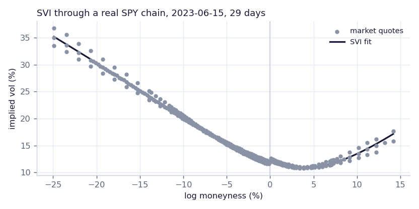
286 real quotes from one SPY expiry, and the five parameter curve through them.
| Measure | Value |
|---|---|
| fit RMSE | 0.460 vol points |
| at the money | 11.91% |
| 10% out of the money put | 20.20% |
| skew, put over ATM | 8.3 vol points |
Half a volatility point of error across 286 quotes is a good fit, and the chart shows why: the market is genuinely smooth here, and five parameters are enough to catch it. Notice the shape. Downside is not slightly dearer, it is nearly double, 20.20% against 11.91% at the money. That is the crash premium priced in, and it is the reason a naked short put and a short straddle are completely different trades despite both being short volatility.
What you do with the fitted curve. Once you have vol_at, you can read the volatility of a strike that was never quoted, which is how you price a spread whose wing sits between two listed strikes. Fit it on consecutive days and the parameter path tells you whether the market repriced the level, the slope or the tilt, which is more informative than watching a single at the money number move.
Five parameters will fit almost any set of points, which says nothing about whether the parameters are identified. Worth measuring rather than asserting, so: take one rich chain, draw random subsets of it, refit, and watch how much rho moves. 300 draws per size, on a free Cboe SPY chain with 284 quotes at 46 days.
# pip install scipy pandas numpy
import numpy as np, pandas as pd
from scipy.optimize import least_squares
rng = np.random.default_rng(7)

# ---------- data collection: one live chain from Cboe, no account, no key ----------
import json, urllib.request
url = "https://cdn.cboe.com/api/global/delayed_quotes/options/SPY.json"
raw = json.loads(urllib.request.urlopen(
    urllib.request.Request(url, headers={"User-Agent": "Mozilla/5.0"}), timeout=90).read())
spot = float(raw["data"]["current_price"])

import re
OCC = re.compile(r"^([A-Z^_]+?)(\d{6})([CP])(\d{8})$")
rows = []
for c in raw["data"]["options"]:
    m = OCC.match(c["option"])
    if not m or not c["iv"] or c["bid"] <= 0:      # iv==0 means Cboe did not solve it
        continue
    rows.append(dict(expiry=pd.Timestamp.strptime(m.group(2), "%y%m%d"),
                     strike=int(m.group(4)) / 1000, side=m.group(3), iv=c["iv"]))
d = pd.DataFrame(rows)
d["dte"] = (d.expiry - pd.Timestamp.today().normalize()).dt.days
d = d[((d.strike >= spot) & (d.side == "C")) | ((d.strike < spot) & (d.side == "P"))]  # OTM side

g = d[d.dte == 46]
T = 46 / 365
k_all, w_all = np.log(g.strike / spot).values, (g.iv.values ** 2) * T


def svi(p, k):
    a, b, rho, m, s = p
    return a + b * (rho * (k - m) + np.sqrt((k - m) ** 2 + s ** 2))


def fit(k, w):
    r = least_squares(lambda p: svi(p, k) - w, [w.mean(), .1, -.5, 0., .1],
                      bounds=([-np.inf, 0, -.999, -np.inf, 1e-6],
                              [np.inf, np.inf, .999, np.inf, np.inf]), max_nfev=20000)
    return r.x


for n in (10, 16, 24, 40, 80, 160, len(k_all)):
    rhos = [fit(k_all[i], w_all[i])[2]
            for i in (rng.choice(len(k_all), n, replace=False) for _ in range(300))]
    print(f"n={n:4d}  rho median {np.median(rhos):+.4f}  "
f"5-95 {np.percentile(rhos,5):+.3f} to {np.percentile(rhos,95):+.3f}")| Quotes in the fit | Median rho | 5th to 95th percentile | Width |
|---|---|---|---|
| 10 | -0.0682 | -0.254 to +0.842 | 1.096 |
| 16 | -0.0856 | -0.180 to +0.196 | 0.376 |
| 24 | -0.0895 | -0.191 to +0.029 | 0.220 |
| 40 | -0.1115 | -0.171 to -0.004 | 0.167 |
| 80 | -0.1176 | -0.159 to -0.045 | 0.114 |
| 160 | -0.1219 | -0.146 to -0.076 | 0.070 |
| 284, all of them | -0.1209 | exact | 0 |
At ten quotes the 90% range for rho runs from -0.254 to +0.842. Same chain, same code, same day. One draw says the smile leans to the downside, another says it leans hard the other way, and every one of them produces a curve that looks fine plotted against its own points.
Rho is the skew, so that is the parameter people quote, and on a thin chain it is not measured. It stabilises around 40 to 80 quotes and is solid by 160. Below roughly 24 the fit is decoration.
Note what is not happening: rho never pinned to the boundary of plus or minus 1 in any of the 2,100 refits, and no draw violated the positivity condition. Failure here is not dramatic, which is why it gets missed. Nothing errors, no warning prints, the RMSE stays low, and you get a confident number that would have been different with a different ten strikes. Count your surviving quotes before quoting a skew.
Data used: SPY daily closes from yfinance, 2015 to 2026, 2,910 returns, free. Plus 8 years of Kaggle SPY chains for the implied leg, 1,999 matched days.
Data missing: the full strike strip. Implied series here reads one at the money strike, so it sits about 3.4 points under VIX and the premium below is understated.
This is the one to spend real time on, because it is the only model here that produces the number on the other side of the trade. Everything else prices what the market is charging. GARCH tells you what you should have charged.
Bollerslev's GARCH(1,1) is one equation. Today's variance is a weighted blend of a constant, yesterday's squared surprise and yesterday's variance:
σ2t = ω + α ε2t-1 + β σ2t-1
Three parameters, and two of them carry the meaning. α is how violently variance reacts to a shock. β is how long it remembers. Their sum is persistence, and persistence decides everything downstream:
half life = ln(0.5) / ln(α + β)
Unconditional variance the model implies, the level it drifts back to when nothing happens, is
σ2∞ = ω / (1 − α − β)
which requires α + β < 1. As persistence approaches 1 that denominator approaches zero and the implied long run level explodes. Watch what that does below, because it does it on real data.
Forecasting is the same recursion run forward, and it converges geometrically to the unconditional level:
E[σ2t+h] = σ2∞ + (α + β)h ( σ2t − σ2∞ )
Errors are fitted with a Student t rather than a normal, because equity returns have fat tails and a normal likelihood compensates by pushing α too low.
ω, α and β are not estimated by least squares. Variance is never observed, so there is no residual to square against it. They come from maximum likelihood: choose the parameters that make the returns you actually saw as probable as possible, given that each day's return is drawn from a distribution whose width is set by the recursion above.
rt = μ + εt, εt = σt zt, zt ~ tν standardised to unit variance
Maximise the sum of daily log densities, where σ2t is supplied by the GARCH recursion and therefore depends on every earlier return:
ln L = Σt [ ln fν( εt / σt ) − ½ ln σ2t ]
That second term is doing the real work and is worth pausing on. Without it, the likelihood would be maximised by making σt enormous, since a wide distribution never finds any observation surprising. Subtracting ln σ2t penalises claiming volatility you did not need, so the fit is a trade between explaining the big days and not over insuring the quiet ones.
With Student t errors the density carries the tail parameter ν, estimated alongside:
fν(z) ∝ ( 1 + z2 / (ν − 2) )-(ν+1)/2
As ν → ∞ this collapses to the normal. Fitted on SPY it lands near 5, meaning fourth moments barely exist. That matters for α: under a normal likelihood a minus 8% day is so improbable that the optimiser inflates the baseline variance to accommodate it, dragging α down and flattening the whole reaction. A t distribution can absorb that day in its tail and leave the dynamics alone.
Why the code multiplies returns by 100. Not cosmetic. Daily log returns are around 0.01, so their squares are around 1e-4 and ω comes out near 1e-6. Quasi Newton optimisers work on finite difference gradients with a fixed step, and at that scale the gradient is numerical noise, so the fit either fails to converge or stops early at a wrong answer. Rescaling to percent moves the parameters into a range where the optimiser behaves. arch warns about it, and the warning is worth obeying.
Written as functions because you will want to run it on more than one ticker, and because the forecast step is the part you will keep.
# pip install arch yfinance pandas numpy
import numpy as np, pandas as pd, yfinance as yf
from arch import arch_model


def returns(ticker="SPY", start="2015-01-01", end="2026-08-01"):
    """Percent log returns. arch wants percent, not decimals, or the optimiser struggles."""
    px = yf.download(ticker, start=start, end=end, progress=False,
                     auto_adjust=True)["Close"].squeeze()
    return (100 * np.log(px / px.shift(1)).dropna())


def fit_garch(r, dist="t"):
    """GARCH(1,1) with Student t errors. The t matters: equity returns have fat tails and
    a normal likelihood pushes alpha too low to compensate."""
    return arch_model(r, vol="GARCH", p=1, q=1, dist=dist).fit(disp="off")


def describe(res):
    p = res.params
    persist = p["alpha[1]"] + p["beta[1]"]
    return {
        "alpha": p["alpha[1]"],                       # reaction
        "beta": p["beta[1]"],                         # memory
        "persistence": persist,
        "half_life_days": np.log(0.5) / np.log(persist),
        "uncond_vol": np.sqrt(p["omega"] / (1 - persist) * 252),
    }


def forecast_vol(res, horizon=21):
    """Annualised vol path. horizon=21 is one option month."""
    f = res.forecast(horizon=horizon, reindex=False)
    return np.sqrt(f.variance.values[-1] * 252)


def realised_vol(r, window=21):
    """Trailing realised, for comparison. Same units as the forecast."""
    return (r / 100).rolling(window).std() * np.sqrt(252) * 100


if __name__ == "__main__":
    r = returns("SPY")
    res = fit_garch(r)
    d = describe(res)
    print(f"alpha {d['alpha']:.4f}   beta {d['beta']:.4f}")
    print(f"persistence {d['persistence']:.4f}   half life {d['half_life_days']:.1f} days")
    print(f"implied unconditional vol {d['uncond_vol']:.1f}%")
print("21 day forecast:", forecast_vol(res, 21).round(1)[:5], "...")| Parameter | Value | What it means |
|---|---|---|
| alpha | 0.1683 | reaction to yesterday's shock |
| beta | 0.8256 | memory of yesterday's variance |
| alpha + beta | 0.9939 | persistence |
| half life | 113.5 days | time for a vol shock to half decay |
| implied unconditional vol | 30.5% | wrong, and instructive, see below |
Persistence of 0.9939 is the headline. A volatility shock takes about 113 days to half fade. If you sell premium after a spike because "it always calms down", that is the number telling you calm is a quarter away, not a fortnight.
And the model tells you where it breaks. With persistence that close to 1 the process is nearly integrated, so the unconditional volatility it implies comes out at 30.5% annualised, which is obviously wrong for SPY. That is not a coding error, it is the known failure of GARCH on long equity samples. Use it for the short horizon forecast, ignore its long run mean.
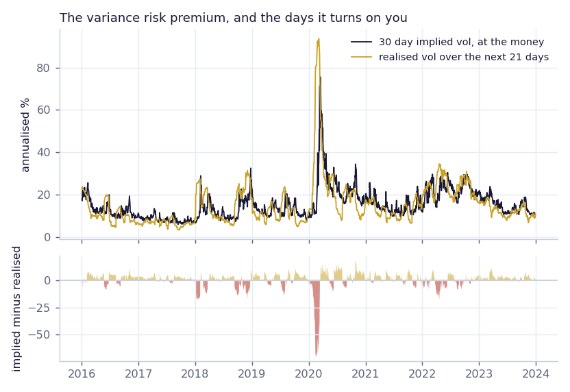
A vol forecast on its own is trivia. It becomes a trade when you put it next to what the market is charging, and the difference has a name: the variance risk premium. Sell an option and you are paid implied volatility. What you owe is whatever volatility actually turns up before expiry. That gap is the edge, and its shape is the whole story.
So this compares 30 day at the money implied vol from the historical chains against the volatility that actually arrived over the following 21 trading days.
# pip install kagglehub arch yfinance pandas numpy pyarrow
from pathlib import Path
import numpy as np, pandas as pd, yfinance as yf

# ---------- data collection: Kaggle as an API call, not a manual download ----------
# needs a free Kaggle token, either ~/.kaggle/kaggle.json or the env vars
# KAGGLE_USERNAME / KAGGLE_KEY. 14 parquet files, about 600 MB, cached after the
# first call so re-running costs nothing.
import kagglehub
KAGGLE = Path(kagglehub.dataset_download(
    "dudesurfin/spy-options-eod-volatility-surface-2010-2023"))
# -> spy_eod_2010.parquet ... spy_eod_2023.parquet


def atm_implied(years=range(2016, 2024), dte=(25, 35)):
    """30 day at the money implied vol, one point per day, from the Kaggle SPY chains.
    Averaging the call and put IV at the nearest strike cancels most of the
    put call parity noise you get in a free end of day snapshot."""
    out = []
    for y in years:
        f = KAGGLE / f"spy_eod_{y}.parquet"
        if not f.exists():
            continue
        d = pd.read_parquet(f)
        d.columns = [c.strip().strip("[]") for c in d.columns]
        for c in ("UNDERLYING_LAST", "STRIKE", "DTE", "C_IV", "P_IV"):
            d[c] = pd.to_numeric(d[c], errors="coerce")
        d["QUOTE_DATE"] = pd.to_datetime(d["QUOTE_DATE"])
        d = d[d.DTE.between(*dte)].copy()
        d["dist"] = (d.STRIKE - d.UNDERLYING_LAST).abs()
        atm = d.loc[d.groupby("QUOTE_DATE").dist.idxmin()]        # nearest strike each day
        out.append(atm.set_index("QUOTE_DATE")[["C_IV", "P_IV"]].mean(axis=1) * 100)
    iv = pd.concat(out).sort_index()
    return iv[(iv > 3) & (iv < 90)].rename("iv")                   # drop solver blow-ups


def forward_realised(ticker="SPY", window=21):
    """Realised vol over the NEXT `window` days. This is what the option pays against,
    and using trailing realised here instead is the most common mistake in this analysis."""
    px = yf.download(ticker, start="2015-12-01", end="2024-03-01",
                     progress=False, auto_adjust=True)["Close"].squeeze()
    lr = np.log(px / px.shift(1)).dropna()
    fwd = lr[::-1].rolling(window).std()[::-1].shift(-1)
    return (fwd * np.sqrt(252) * 100).rename("realised_fwd")


iv, fwd = atm_implied(), forward_realised()
j = pd.concat([iv, fwd], axis=1).dropna()
j["vrp"] = j.iv - j.realised_fwd

print(f"mean premium   {j.vrp.mean():+.2f} vol points")
print(f"median premium {j.vrp.median():+.2f}")
print(f"positive on    {100*(j.vrp>0).mean():.1f}% of days")
print(f"worst day      {j.vrp.min():.1f} on {j.vrp.idxmin().date()}")
1,999 trading days, 2016 to 2023. Gold is premium earned, red is premium paid.
| Measure | Value |
|---|---|
| mean implied | 15.37% |
| mean realised, forward | 15.11% |
| mean premium | +0.27 vol points |
| median premium | +1.62 vol points |
| positive on | 67.0% of days |
| worst day | -69.7 on 19 February 2020 |
Look at the mean against the median. The median premium is +1.62 volatility points and it is positive on two days out of three. Mean is +0.27. That entire gap is a handful of days, and it is the most important thing on this page.
Selling volatility works most of the time and then hands back years of it in a fortnight. Worst observation is 19 February 2020, which was the exact top before the COVID crash: implied was around 14% and the following month realised over 80%. One day, minus 69 volatility points. That single episode is what drags a comfortable +1.62 median down to a barely there +0.27 mean.
Which is why GARCH earns its place. It will not predict 19 February 2020, nothing will. What it gives you is persistence, and persistence tells you that after the shock arrives, vol stays elevated for about 113 days, so the recovery trade is slower than instinct suggests. Forecasting is not the edge. Knowing the shape of the loss is.
Data used: none for the pricing itself. Inputs below are the real 15 June 2023 SPY chain, spot 442.61 and 11.91% vol, so the numbers connect to the rest of the page.
Data missing: nothing for this section. What it does need is a GPU, and on native Windows that is not available, see the honest note at the end.
CUDA and a GPU pay off on large data sets, and specifically on large scale research, calibration and risk management. Those three share the property that makes this library worth the dependency: you know every contract you need to price before you start, so they can all go through in one batch. At a few hundred contracts the library is worth nothing. At hundreds of thousands it is a different category of tool, and the evidence below is Google's own American option example run against QuantLib on this machine.
This is the one library here that is not a new model. Google published no new mathematics. What they published is the same mathematics expressed as tensor operations, so that pricing a million contracts is one array instruction instead of a million function calls.
Maths being vectorised is Black and Scholes, so it is worth writing down properly, because the reason it vectorises so well is visible in the equations. A European call is
C = e-rT [ F Φ(d1) − K Φ(d2) ]
F = S e(r − q)T
d1 = [ ln(F/K) + ½σ2T ] / (σ√T) d2 = d1 − σ√T
Every symbol on the right is either a scalar or a per contract number, and there is no loop, no recursion and no path dependence anywhere in it. Change K from a number to an array of a million strikes and the formula is unchanged, which is exactly the property a GPU exploits. A closed form price is embarrassingly parallel by construction.
Why anyone cares. Not to price one option, which any library does instantly. Calibration is the reason. Fitting Heston to a chain means repricing the whole surface a few thousand times while an optimiser searches five parameters, which is what the QuantLib section below actually does. Repricing is the inner loop, so making the inner loop a single tensor operation is the difference between a calibration that finishes and one you abandon.
# pip install tf-quant-finance tensorflow tf-keras
# TensorFlow 2.21 supports Python 3.10 to 3.13 ONLY. On 3.14 pip reports
# "no matching distribution found", which reads like a broken index.
import tf_quant_finance as tff

tff.black_scholes.option_price(...)          # vanilla European, vectorised
tff.black_scholes.implied_vol(...)           # inverts the above, also vectorised
tff.models.heston.HestonModel(...)           # stochastic vol, Monte Carlo or PDE
tff.math.pde.fd_solvers.solve_backward(...)  # the finite difference engine
tff.math.random.multivariate_normal(...)     # low discrepancy sequences for MC

# every argument is an ARRAY. one option and a million options are the same call.This prices the same contracts two ways, tf-quant-finance against a hand written scipy implementation, and times both at three sizes. Comparison is the point, because it tells you where the library starts being worth the dependency.
# pip install tf-quant-finance tensorflow tf-keras scipy numpy
import os, time
os.environ["TF_CPP_MIN_LOG_LEVEL"] = "3"
os.environ["PROTOCOL_BUFFERS_PYTHON_IMPLEMENTATION"] = "python"   # else protobuf errors
import numpy as np, tensorflow as tf, tf_quant_finance as tff
from scipy.stats import norm

# no download here on purpose: the inputs below are the real 15 June 2023 SPY
# chain, hard coded so the benchmark reproduces without fetching anything.

# the real 15 June 2023 SPY chain, so this ties to the rest of the page
SPOT, VOL, T, R, Q = 442.61, 0.1191, 29 / 365, 0.05, 0.015


def tff_price(strikes):
    """Google's implementation. Every argument is an array of the same length."""
    n = len(strikes)
    return tff.black_scholes.option_price(
        volatilities=np.full(n, VOL),
        strikes=strikes,
        expiries=np.full(n, T),
        spots=np.full(n, SPOT),
        discount_rates=np.full(n, R),
        dividend_rates=np.full(n, Q),
        is_call_options=strikes >= SPOT).numpy()


def scipy_price(strikes):
    """The same closed form, written out, as the control."""
    F = SPOT * np.exp((R - Q) * T)
    df = np.exp(-R * T)
    s = VOL * np.sqrt(T)
    d1 = (np.log(F / strikes) + 0.5 * s * s) / s
    d2 = d1 - s
    call = df * (F * norm.cdf(d1) - strikes * norm.cdf(d2))
    put = df * (strikes * norm.cdf(-d2) - F * norm.cdf(-d1))
    return np.where(strikes >= SPOT, call, put)


for n in (1_000, 100_000, 1_000_000):
    k = np.linspace(300.0, 600.0, n)
    tff_price(k[:10])                                   # warm the graph, or you time the compile
    t0 = time.perf_counter(); a = tff_price(k)
    t1 = time.perf_counter(); b = scipy_price(k)
    t2 = time.perf_counter()
    print(f"{n:9d} options   tff {1000*(t1-t0):7.1f} ms   "
f"scipy {1000*(t2-t1):7.1f} ms max diff {np.abs(a-b).max():.1e}")| Contracts | tf-quant-finance | scipy | Speed up | Max difference |
|---|---|---|---|---|
| 1,000 | 2.6 ms | 2.3 ms | 0.9x, slower | 1.1e-13 |
| 100,000 | 22.5 ms | 33.5 ms | 1.5x | 1.6e-13 |
| 1,000,000 | 130.4 ms | 422.9 ms | 3.2x | 1.8e-13 |
First row decides whether you need this at all. At a thousand contracts the library is slower than fifteen lines of scipy, because you are paying graph construction overhead to save arithmetic that was never expensive.
Crossover sits somewhere around a hundred thousand. At a million contracts it is 3.2 times faster and prices roughly 7.7 million options a second on a laptop CPU. That is the regime calibration lives in, and it is the only regime where this dependency earns its place.
Agreement between them is worth noting too. Maximum difference of 1.8e-13 across a million contracts is floating point noise, so the two implementations are the same formula and the comparison is purely about speed.
Everything above is a benchmark written here, which is fair but is not theirs. So this is their code: the american_option finite difference pricer lifted unchanged out of American_Option_Black_Scholes.ipynb, priced against QuantLib's own finite difference engine on the same contracts. Their notebook runs exactly this comparison, which is what makes it the honest test.
# pip install tf-quant-finance tensorflow tf-keras QuantLib
import tensorflow as tf
from tf_quant_finance.math import pde


@tf.function
def american_option(number_grid_points, time_delta, strike, volatility,
                    risk_free_rate, expiry, dtype=tf.float64):
    s_min, s_max = 0.01, 300.
    grid = pde.grids.uniform_grid(minimums=[s_min], maximums=[s_max],
                                  sizes=[number_grid_points], dtype=dtype)
    final_values_grid = tf.nn.relu(grid[0] - strike)

    def second_order_coeff_fn(t, grid): return [[volatility**2 * grid[0]**2 / 2]]
    def first_order_coeff_fn(t, grid):  return [risk_free_rate * grid[0]]
    def zeroth_order_coeff_fn(t, grid): return -risk_free_rate

    # this is what makes it AMERICAN: after every backward step, floor the value at
    # the intrinsic payoff. that single line is the early exercise decision.
    def values_transform_fn(t, grid, values):
        return grid, tf.maximum(values, tf.nn.relu(grid[0] - strike))

    v, g, _, _ = pde.fd_solvers.solve_backward(
        start_time=expiry, end_time=0, coord_grid=grid,
        values_grid=final_values_grid, time_step=time_delta,
        values_transform_fn=values_transform_fn, ...)
    return v, g[0]

# strike, volatility and risk_free_rate are all (n, 1) tensors.
# ONE call prices n contracts. that is the entire trick.
What is being solved backwards is Black and Scholes in differential form, which is where those three coefficient functions come from:
∂V/∂t + ½σ2S2 ∂2V/∂S2 + rS ∂V/∂S − rV = 0
Second order coefficient, first order coefficient, zeroth order coefficient. They map one to one onto the code, which is the clearest case on this page of a library mirroring its own mathematics rather than hiding it.
| Contracts | tf-quant-finance | QuantLib | Speed up |
|---|---|---|---|
| 1 | 59 /sec | 43 /sec | 1.4x |
| 50 | 961 /sec | 550 /sec | 1.7x |
| 200 | 2,642 /sec | 533 /sec | 5.0x |
| 1,000 | 2,251 /sec | 567 /sec | 4.0x |
QuantLib flatlines around 550 a second and never improves, because a loop over contracts amortises nothing. tf-quant-finance climbs to roughly 2,600 and holds there. Worth noticing: Google's notebook quotes about 3,000 American options a second for a GPU, and this machine reached 2,642 on the CPU. Batching is doing most of the work, and the device is only the last multiple.
Specific to this machine rather than a general remark. Card is an RTX 4050 Laptop GPU, 6 GB, driver 591.94, compute capability 8.9, which is perfectly capable of running all of this. TensorFlow refuses anyway:
WARNING:tensorflow: TensorFlow GPU support is not available on native Windows
for TensorFlow >= 2.11. Even if CUDA/cuDNN are installed, GPU will not be used.
Please use WSL2 or the TensorFlow-DirectML plugin.

>>> tf.test.is_built_with_cuda()
False
>>> tf.config.list_physical_devices()
['CPU']          # the 4050 is invisible by design, not by fault
On native Windows the choices are WSL2, where the CUDA build works properly, or pinning TensorFlow 2.10, the last native Windows release with GPU support and now too old for current tf-quant-finance. Every number above is a CPU floor with the 4050 sitting idle.
One version trap that cost an install. TensorFlow 2.21 supports Python 3.10 to 3.13. On Python 3.14 pip reports "no matching distribution found", which reads like a broken package index rather than an unsupported interpreter. Everything here ran on 3.11.
Four jobs, all of them large data set jobs:
All four know every contract they need to price before they start, which is the condition batching requires. Where that condition fails, and you need one price right now rather than ten million prices soon, the graph overhead in the first row of the benchmark is a cost with nothing on the other side.
Data used: the Kaggle SPY chain for 15 June 2023, spot 442.61. 72 quotes across 8 expiries from 25 to 180 days, within 12% of the money.
Data missing: a real rate and dividend curve, flat 5.0% and 1.5% used instead, and the bid ask spreads to weight the fit by.
Black and Scholes assumes volatility is a constant. It is not, and the evidence is that the market charges different volatilities for different strikes on the same underlying and the same day. Heston's 1993 answer is to let variance be random and give it its own equation. Two processes, driven by two correlated shocks:
dSt = μSt dt + √vt St dWSt
dvt = κ(θ − vt) dt + σ√vt dWvt
d⟨WS, Wv⟩t = ρ dt
Five parameters, and each one has a job you can see in the smile:
That last point is the reason Heston matters and the reason it is not SVI. SVI describes a smile with a formula that fits well. Heston explains the smile as a consequence of variance being random and negatively correlated with returns. One is a curve fit, the other is a mechanism, and only the mechanism prices a path dependent product.
Variance here follows a CIR process, which carries a condition. Feller:
2κθ > σ2
If it holds, variance can never reach zero. If it fails, variance touches zero and reflects. Remember this, because the calibration below breaks it.
Heston is famous because it is a stochastic volatility model you can still price almost analytically. Most are not, and need Monte Carlo, which puts calibration out of reach. What makes Heston different is that while the density of log spot has no closed form, its characteristic function does:
φT(u) = E[ eiu ln ST ] = exp( C(u,T) + D(u,T) v0 + iu ln F )
where C and D solve a pair of Riccati ordinary differential equations that have explicit solutions. D carries the initial variance and C accumulates the drift of the variance process:
D(u,T) = ( (κ − iρσu − d) / σ2 ) · ( 1 − e-dT ) / ( 1 − g e-dT )
d = √( (ρσu i − κ)2 + σ2(iu + u2) )
Price then comes from a single numerical integral rather than a simulation:
C = S e-qT P1 − K e-rT P2
Pj = ½ + (1/π) ∫0∞ Re[ e-iu ln K φj(u) / (iu) ] du
That integral is what AnalyticHestonEngine evaluates. It costs microseconds, which is the only reason a five parameter search over 72 quotes finishes in seconds instead of hours. Swap in MCEuropeanHestonEngine and the same calibration becomes an overnight job.
One numerical trap worth knowing, and it is the classic Heston bug rather than an implementation slip. That square root d is complex, and the naive branch of the complex logarithm inside C jumps discontinuously for long maturities, which makes prices oscillate wildly past roughly two years. Known as the Heston trap, solved by Albrecher's "little trap" formulation. QuantLib already uses the stable branch, so it is invisible here, and it is the reason to use their engine rather than typing the formula out yourself.
Calibration is not fitting a curve through implied vols. Each HestonModelHelper converts your quoted vol into a Black and Scholes price, then compares that to the Heston price of the same contract. What the optimiser minimises is
minΘ Σi wi ( PHestoni(Θ) − Pmarketi )2, Θ = (v0, κ, θ, σ, ρ)
and calibrationError() reports the relative version, price error divided by market price. This detail decides the answer. Errors in price weight at the money contracts heavily, because they are worth the most, while a wing option worth 30 cents contributes almost nothing however wrong it is in vol terms. Fit the same chain in vol space and you get different parameters from the same data.
Hence the unweighted least squares warning in the curation step. Every wi here is 1, so the fit is already tilted toward the money before any filtering, and the honest improvement is to weight by vega or by inverse spread so each quote counts in proportion to how much it can be trusted.
Five parameters and a non convex surface means the optimiser finds a minimum, not the minimum. Starting from a different guess can land somewhere else, which is why the run below is repeated from several starting points and why the resulting parameters should be read as one plausible description of the surface rather than as measurements.
# pip install QuantLib
import QuantLib as ql

ql.HestonProcess(rf, div, spot, v0, kappa, theta, sigma, rho)
ql.HestonModel(process)
ql.AnalyticHestonEngine(model)          # semi closed form, fast enough to calibrate
ql.HestonModelHelper(tenor, cal, spot, strike, vol_quote, rf, div)
model.calibrate(helpers, ql.LevenbergMarquardt(), ql.EndCriteria(...), constraint)

# THE TRAP: model.params() returns theta, kappa, sigma, rho, v0
# NOT the constructor order v0, kappa, theta, sigma, rho. Unpacking positionally
# gives a plausible looking set of numbers that are completely wrong.
That comment cost two bad calibrations, and then a third. params() and the HestonProcess constructor use different orders, so reading the result positionally gives five plausible numbers that are wrong. Surest check is to build a process with five distinct dummy values and read back what params() returns.
Same ordering bites a second time, on the constraint, and there it fails silently. NonhomogeneousBoundaryConstraint also takes its bounds in params() order. Supply them in constructor order and rho inherits a lower bound of 1e-4 while v0 inherits an upper bound of 0, so the starting point is infeasible. LevenbergMarquardt then returns without taking a step and params() hands back the initial guess, which reads exactly like a converged fit. Verify by checking the error actually fell:
err = lambda: 100 * np.mean([abs(h.calibrationError()) for h in helpers])
before = err()
model.calibrate(...)
print(f"{before:.2f}% -> {err():.2f}%")     # 35.15% -> 10.29%. if it does not move, it did not run
Swapping in ql.Simplex(0.05) is the fastest way to expose it, because Simplex raises Initial guess [ 0.03; 3; 0.6; -0.75; 0.03 ] is not in the feasible region and that printed vector tells you the true parameter order directly.
# pip install QuantLib kagglehub pandas numpy pyarrow
from pathlib import Path
import numpy as np, pandas as pd, QuantLib as ql

# ---------- collection: Kaggle as an API call ----------
import kagglehub
KAGGLE = Path(kagglehub.dataset_download(
    "dudesurfin/spy-options-eod-volatility-surface-2010-2023"))

d = pd.read_parquet(KAGGLE / "spy_eod_2023.parquet")
d.columns = [c.strip().strip("[]") for c in d.columns]
for c in ("UNDERLYING_LAST", "STRIKE", "DTE", "C_IV", "P_IV"):
    d[c] = pd.to_numeric(d[c], errors="coerce")
d = d[pd.to_datetime(d.QUOTE_DATE) == "2023-06-15"]
spot = float(d.UNDERLYING_LAST.iloc[0])

# ---------- curation, four filters that all change the fit ----------
rows = []
for _, x in d.iterrows():
    if not (25 <= x.DTE <= 180):        # under 25d the smile is dominated by pin risk,
        continue                        # over 180d the quotes go stale
    k = np.log(x.STRIKE / spot)
    if abs(k) > 0.12:                   # the far wings have the widest spreads and the
        continue                        # least reliable mids, and they dominate an
                                        # unweighted least squares if you let them
    iv = x.P_IV if x.STRIKE < spot else x.C_IV   # OTM side only, always the liquid one
    if not (0.05 < iv < 1.0):
        continue
    rows.append((int(x.DTE), float(x.STRIKE), float(iv)))

q = pd.DataFrame(rows, columns=["dte", "strike", "iv"]).dropna()
# thin to at most 9 strikes per expiry, so no single dense expiry outvotes the others
q = pd.concat([g.iloc[np.linspace(0, len(g)-1, min(9, len(g))).astype(int)]
               for _, g in q.groupby("dte")], ignore_index=True)

# ---------- QuantLib ----------
today = ql.Date(15, 6, 2023); ql.Settings.instance().evaluationDate = today
cal, dc = ql.TARGET(), ql.Actual365Fixed()
rf = ql.YieldTermStructureHandle(ql.FlatForward(today, 0.050, dc))
dv = ql.YieldTermStructureHandle(ql.FlatForward(today, 0.015, dc))
sh = ql.QuoteHandle(ql.SimpleQuote(spot))

proc = ql.HestonProcess(rf, dv, sh, 0.030, 3.0, 0.030, 0.6, -0.75)   # v0,kappa,theta,sigma,rho
model = ql.HestonModel(proc)
engine = ql.AnalyticHestonEngine(model)

helpers = []
for _, x in q.iterrows():
    h = ql.HestonModelHelper(ql.Period(int(x.dte), ql.Days), cal, spot, float(x.strike),
                             ql.QuoteHandle(ql.SimpleQuote(float(x.iv))), rf, dv)
    h.setPricingEngine(engine)
    helpers.append(h)

# THE SAME TRAP AGAIN, and this time it fails SILENTLY. The constraint vector is in
# params() order, NOT constructor order. Write the bounds in constructor order and the
# starting point lands outside the feasible region, LevenbergMarquardt returns without
# taking a single step, and model.params() hands back your initial guess looking like
# a converged answer. Simplex at least raises "Initial guess is not in the feasible
# region". LM says nothing at all.
LO = [1e-4, 0.5, 1e-4, -0.999, 1e-4]      # theta, kappa, sigma, rho, v0
HI = [1.00, 15.0, 5.00,  0.000, 1.000]

model.calibrate(helpers, ql.LevenbergMarquardt(),
                ql.EndCriteria(1000, 100, 1e-8, 1e-8, 1e-8),
                ql.NonhomogeneousBoundaryConstraint(LO, HI))

theta, kappa, sigma, rho, v0 = model.params()      # <-- NOT constructor order
print(f"v0={v0:.5f} kappa={kappa:.4f} theta={theta:.5f} sigma={sigma:.4f} rho={rho:.4f}")
print(f"  spot vol      {100*np.sqrt(v0):.2f}%")
print(f"  long run vol  {100*np.sqrt(theta):.2f}%")
print(f"  Feller 2*k*theta={2*kappa*theta:.4f} vs sigma^2={sigma**2:.4f}")
print(f" mean relative pricing error {100*np.mean([abs(h.calibrationError()) for h in helpers]):.2f}%")| Parameter | Fitted | Reading |
|---|---|---|
| v0 | 0.01185 | spot volatility 10.89% |
| θ | 0.03126 | long run volatility 17.68% |
| κ | 9.7558 | fast reversion, roughly a 5 week half life |
| σ | 2.2781 | very high vol of vol |
| ρ | -0.5418 | the skew, variance rises when spot falls |
Fitted Heston smile against the real quotes it was calibrated to.
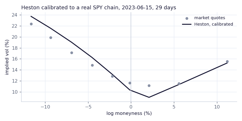
ρ = -0.5418 is the headline and it is the parameter doing the real work. It says the market prices a meaningful negative correlation between returns and variance, which is what makes downside puts expensive. It is not an assumption anyone imposed, it fell out of fitting five numbers to 72 quotes.
v0 at 10.89% against θ at 17.68% says June 2023 was a calm spot priced against a much more volatile long run. That chain expected volatility to roughly double as you look further out, which is the term structure in upward sloping shape, the normal one.
Feller is violated, and badly. 2κθ = 0.6100 against σ2 = 5.1899, a factor of eight the wrong way. Fitted variance can therefore reach zero. This is not a bug in the calibration, it is the standard outcome: fitting Heston to real equity index chains breaks Feller almost every time, because the only way to bend a short dated smile as sharply as the market bends it is to push σ higher than the condition allows. Papers that report a Feller compliant equity fit have usually imposed it as a constraint and accepted a worse fit in exchange.
Practical consequence is narrow but real. It does not affect the vanilla prices here, which come from the semi closed form. It affects Monte Carlo, where a naive Euler discretisation of the variance process will go negative and produce a NaN at the square root. Use the quadratic exponential scheme or full truncation, both of which QuantLib has.
That 10.29% mean relative pricing error is what stops this being a good fit. Five parameters cannot reproduce a whole surface across eight expiries at once. Heston fits any single smile well and struggles to fit the term structure of smiles simultaneously, which is exactly why the industry moved on to local stochastic volatility. If you need to reprice the surface rather than understand it, this section is the wrong tool and SVI, which opens the page, is the right one.
Data used: the same Kaggle SPY chain, 15 June 2023, the 29 day expiry. 109 raw rows, 82 after curation, strikes 385 to 485.
Data missing: nothing needed here. Forward and dividend yield are recovered from the chain itself rather than assumed, which is the point of this section.
No new model. FinancePy's job is the inverse problem and the derivatives. Black and Scholes maps volatility to a price:
C = e-rT [ F Φ(d1) − K Φ(d2) ]
Nobody has a volatility. Everybody has a price. So the useful direction is backwards, solving
find σ such that BS(σ) = Pmarket
which has no closed form and is done by root finding. It works reliably because vega is strictly positive, so the price is monotone in volatility and there is exactly one solution.
Greeks are the derivatives of that same price, and the two that matter for a volatility position are:
ν = ∂C/∂σ = S e-qT φ(d1) √T
Γ = ∂2C/∂S2 = e-qT φ(d1) / (S σ √T)
Both carry φ(d1), a normal density centred at the money, which is why both peak there and decay into the wings. Vega picks up √T and gamma divides by it, so long dated options carry the vega and short dated options carry the gamma. That single fact decides which expiry a volatility view belongs in.
Inverting a chain needs a forward, and using spot is the default mistake. Put call parity gives it back from the quotes themselves:
C − P = e-rT ( F − K )
One caution. Fitting both r and F to 29 day mids does not work, because the regression has almost no leverage on the slope over so short a horizon. Doing it returns a discount factor above 1, a -42.8% interest rate, which is noise wearing a rate's clothes. Pin r at the T-bill and solve for F alone.
# pip install financepy kagglehub pandas numpy pyarrow
from pathlib import Path
import numpy as np, pandas as pd
import kagglehub
from financepy.utils import Date
from financepy.market.curves import DiscountCurveFlat
from financepy.products.equity import EquityVanillaOption
from financepy.utils.global_types import OptionTypes
from financepy.models.black_scholes import BlackScholes

# ---------- curation ----------
d["cmid"] = (d.C_BID + d.C_ASK) / 2
d["pmid"] = (d.P_BID + d.P_ASK) / 2
d = d[d.mid > 0.05]                        # a 1 cent option carries no information
d = d[(d.spread / d.mid) < 0.25]           # relative spread cap, kills the dead wings
d = d[abs(np.log(d.STRIKE / spot)) < 0.15]

# ---------- recover the forward, ONE free parameter ----------
w = d[(abs(np.log(d.STRIKE / spot)) < 0.03) & (d.C_BID > 0) & (d.P_BID > 0)].copy()
df = np.exp(-0.05 * T)
w["F_k"] = w.STRIKE + (w.cmid - w.pmid) / df    # each strike implies a forward
F = float(w.F_k.median())                        # median, so one wide quote cannot move it
q = 0.05 - np.log(F / spot) / T                  # back out the dividend yield

# ---------- invert, then the greeks ----------
val, exp = Date(15, 6, 2023), Date(15, 6, 2023).add_days(29)
disc, divc = DiscountCurveFlat(val, 0.05), DiscountCurveFlat(val, q)

for _, x in d.iterrows():
    call = x.STRIKE >= spot
    o = EquityVanillaOption(exp, float(x.STRIKE),
                            OptionTypes.EUROPEAN_CALL if call else OptionTypes.EUROPEAN_PUT)
    iv = o.implied_volatility(val, spot, disc, divc, float(x.mid))   # the inverse problem
    m = BlackScholes(iv)
    o.value(val, spot, disc, divc, m)
    o.delta(val, spot, disc, divc, m)
    o.gamma(val, spot, disc, divc, m)
    o.vega(val, spot, disc, divc, m)
o.theta(val, spot, disc, divc, m)| Forward used | Correlation | Mean abs error | Puts | Calls |
|---|---|---|---|---|
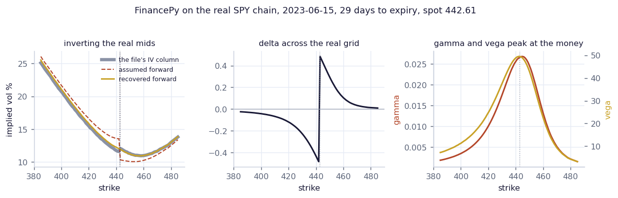
| assumed, spot grown at r − q = 3.5% → 443.843 | 0.98022 | 1.090 pts | +1.185 | -0.908 |
| recovered from parity → 442.257 | 0.99923 | 0.277 pts | +0.388 | -0.036 |
That assumed forward was 36 basis points too high, and that alone put a full volatility point of error into the smile, with the sign flipping between puts and calls. A forward that is too high makes calls look cheap in volatility terms and puts look expensive, which is exactly the signature in the first row. Recovering it cuts the error by a factor of four.
Recovered dividend yield comes out at 6.01% against the 1.5% assumed, which is not a real dividend forecast. It is the parity residual absorbing the borrow cost, the discrete June dividend and the early exercise value of an American option, all of which the European formula has nowhere else to put. It is a plug, and the honest way to read it is as the number that makes the chain internally consistent rather than as a forecast of SPY's payout.
Left, the same smile inverted three ways. Middle and right, their greeks across the real strike grid.
Kaggle's file ships precomputed greeks, so the library can be checked against a completely independent implementation on the same contracts.
| Greek | Correlation | File / FinancePy | What the ratio means |
|---|---|---|---|
| delta | 1.00000 | 0.9874 | same convention |
| gamma | 0.99996 | 0.9803 | same convention |
| vega | 1.00000 | 0.0101 | the file quotes per 1% of vol, FinancePy per 1.00 |
| theta | 0.99995 | 0.0026 | the file quotes per day, FinancePy per year |
Correlations of 0.9999 and above on all four, so the mathematics agrees exactly. Ratios are what to take away. 0.0101 is 1/99 and 0.0026 is 1/385, near enough to 1/100 and 1/365 to be certain what happened: the two implementations disagree only on units. Vega per volatility point against vega per unit of volatility, theta per day against theta per year. Nobody is wrong and a position sized off the mismatch is wrong by a hundred times.
Numbers on their own do not mean much, so here they are as a trade. 100 lots of the 25 delta put, the standard downside hedge.
| Measure | Value | What it means |
|---|---|---|
| premium | $24,800 | what it costs |
| delta hedge | -2,428 shares | sell this much SPY to be flat direction |
| gamma | +184.5 | the hedge needs 185 shares adjusting per $1 move |
| vega | +$3,895 | per volatility point, so 13.56% to 14.56% is +$3,895 |
| theta | -$937 | bled every day nothing happens |
Set gamma against theta and the position states its own terms. Daily move that pays for the decay is
ΔS = √( 2 × |θdaily| / Γ )
which here is $3.19, or 0.72% of spot, every single day. Realised volatility of about 11.4% annualised. That option was bought at an implied 13.56%, so the trade is the variance risk premium from the other side, and it is the same premium measured in the arch section above. Long volatility is short carry, and this is the exchange rate between the two.
Data used: SPY, TLT and nine G10 currency pairs from yfinance, 2010 to 2024, free and no account.
Data missing: a Marquee client id and secret, which unlocks their pricing engine and their implied volatility surfaces.
Their analytics run locally and you can reach effectively the same answers with free data. gs-quant is three things and only two are gated. gs_quant.markets and gs_quant.instrument, the pricing engine, need a session. gs_quant.data, their market data, needs a session. gs_quant.timeseries, the analytics, does not. It is pure functions over pandas objects, computed on your machine, and it accepts whatever series you hand it.
That boundary is per function and undocumented, so it is worth knowing where it falls.
| Runs offline | Needs a GsSession |
|---|---|
volatility, exponential_volatility, correlation, covariance, beta, max_drawdown, percentiles, percentileofscore, zscores, winsorize, smooth_spikes, returns | semi_variance, realized_volatility, every implied_volatility variant, var_swap, forward_vol, the whole rates and FX curve family |
Pattern is simple: anything computed from a series you supply is free, and anything that needs to fetch a surface or a curve is not.
No stochastic model here. These are estimators, and the value is that the conventions are fixed rather than reinvented per analyst.
rt = ln( Pt / Pt-1 )
σW = √252 × stdev( rt-W+1 … rt ) × 100
That square root of 252 assumes returns are independent across days. They are not, which is the subject of the arch section above, so this is a convention rather than a truth. Everyone uses it, which is what makes it comparable.
Their exponentially weighted version drops the fixed window and decays instead, which reacts faster to a shock:
σ2t = λ σ2t-1 + (1 − λ) r2t, λ = 0.94
And correlation and beta, which is correlation scaled by the volatility ratio:
ρW = cov( rA, rB ) / ( σA σB ) βA|B = ρ × ( σA / σB )
Window(size, ramp) takes a ramp up as its second argument, how many observations to discard before emitting. It defaults to the window size. Passing 0 emits as soon as it mathematically can, which means the first values are unreliable and you trim them yourself.
# pip install gs-quant
# installs and imports with no credentials. 46 of its 48 timeseries functions
# run fully offline, see the table above.
import gs_quant.timeseries as ts
from gs_quant.timeseries import Window

ts.volatility(px, Window(63, 0))          # annualised, already in percent
ts.exponential_volatility(px, 0.94)       # EWMA, RiskMetrics decay
ts.correlation(a, b, Window(63, 0))       # rolling pairwise
ts.beta(a, b, Window(63, 0))              # a regressed on b
ts.percentiles(series, w=Window(504, 0))  # rank against its own trailing 2 years
ts.max_drawdown(px, Window(252, 0))
ts.smooth_spikes(px, 0.10)                # their own bad print filter

# no GsSession anywhere. nothing leaves the machine.Rather than invent an example, the repo ships one: gs_quant/content/reports_and_screens/00_fx/vol_screen_app.py. It is a G10 volatility monitor, and its g10 list is exactly these nine pairs. Their function, unedited:
# gs_quant/content/reports_and_screens/00_fx/vol_screen_app.py, theirs
def volatility_screen(crosses, start_date, end_date, tenor='3m', plot=True):
    fxspot_dataset, fxvol_dataset = Dataset('FXSPOT'), Dataset('FXIMPLIEDVOL')
    for cross in crosses:
        spot = fxspot_dataset.get_data(start_date, end_date, bbid=cross)[['spot']]
        spot_data[cross] = volatility(spot['spot'], tenor)          # realized
        vol = fxvol_dataset.get_data(..., tenor=tenor, deltaStrike='DN', location='NYC')
        impvol_data[cross] = vol.drop_duplicates(keep='last') * 100  # implied

    spdata, ivdata = format_df(spot_data), format_df(impvol_data)
    diff = ivdata.subtract(spdata).dropna()
    ...
        data[cross] = {'Spot': last_value(spot_fx[cross]),
                       '{} Implied'.format(tenor): last_value(ivdata[cross]),
                       '{} Realized'.format(tenor): last_value(spdata[cross]),
                       'Diff': last_value(diff[cross]),
                       'Historical Implied Low': min(ivdata[cross]),
                       'Historical Implied High': max(ivdata[cross]),
                       '%-ile': last_value(percentiles(ivdata[cross]))}

g10 = ['USDJPY', 'EURUSD', 'AUDUSD', 'GBPUSD', 'USDCAD',
       'USDNOK', 'NZDUSD', 'USDSEK', 'USDCHF']
Two data pulls. FXSPOT has a free substitute in yfinance. FXIMPLIEDVOL does not, so the implied leg is replaced with forward realised volatility, the quantity implied is trying to forecast. Everything else, the tenor string, the column names, format_df, percentiles, last_value and the scatter, is kept as they wrote it.
Notice they pass tenor='3m', a string, rather than the Window(63, 0) form used above. Their functions accept a relative date and convert it, which is the more idiomatic call.
Their helper ends with .ffill().dropna(), which is right for two contemporaneous market series and is what they feed it. It is wrong for a forward looking leg. Forward realised is unobservable over the last 63 days, so ffill carries the last known value across that tail and the screen date ends up reading its own trailing volatility. Diff comes out as exactly 0.00 for all nine pairs, which looks like a plausible answer rather than an obvious failure.
# their format_df, kept, because for their own inputs it is correct
def format_df(data_dict):
    df = pd.concat(data_dict, axis=1)
    df.columns = data_dict.keys()
    return df.ffill().dropna()

spdata = format_df(spot_data)          # their line, safe here
ivdata = spdata.shift(-63)             # forward leg built AFTER the align, never ffilled
asof = ivdata.dropna(how="any").index[-1]   # last date the forward window is complete
diff = (ivdata - spdata).dropna(how="any")
Screen is therefore dated at the last fully observable point rather than at today. Reporting it as of today would require the future.
Free FX data carries bad prints. USDNOK printed 10.78, then 7.74, then 11.76 on consecutive days in March 2020, a 35% round trip that cannot happen in G10. One bad price creates two bad returns, going in and coming out, and it pushed the maximum 3 month volatility for that pair to 120.46.
Repo ships three cleaners, so the honest move is to compare them rather than write a fourth.
# pip install gs-quant yfinance pandas numpy
import pandas as pd, yfinance as yf
import gs_quant.timeseries as ts
from gs_quant.timeseries import volatility, percentiles, last_value, Window

# ---------- data collection: the nine G10 pairs, free, no account ----------
PAIRS = {c: (c[3:] + "=X" if c.startswith("USD") else c + "=X") for c in
         ['USDJPY','EURUSD','AUDUSD','GBPUSD','USDCAD','USDNOK','NZDUSD','USDSEK','USDCHF']}
raw = yf.download(list(PAIRS.values()), start="2018-01-01", end="2024-01-01",
                  progress=False, auto_adjust=True)["Close"]
raw.columns = [{v: k for k, v in PAIRS.items()}[c] for c in raw.columns]

n = raw["USDNOK"].dropna()
pd.DataFrame({
    "raw":             volatility(n, "3m"),
    "smooth_spikes":   volatility(ts.smooth_spikes(n, 0.10), "3m"),
    "smooth_outliers": volatility(ts.smooth_outliers(n, 0.5), "3m"),
    "winsorize":       volatility(ts.prices(ts.winsorize(ts.returns(n), 2.5, Window(252, 0))), "3m"),
}).describe()| Cleaner | Mean | Std dev | Max | Days changed |
|---|---|---|---|---|
| raw | 18.36 | 22.54 | 120.46 | 0 |
smooth_spikes(0.10) | 12.43 | 4.06 | 26.43 | 198 |
smooth_outliers(0.5) | 18.36 | 22.54 | 120.46 | 0 |
winsorize(2.5) | 12.85 | 4.18 | 26.16 | 255 |
smooth_spikes replaced three prints and cut the maximum from 120.46 to 26.43, touching only USDNOK and leaving the other eight pairs bit for bit identical. winsorize lands in the same place by a different route, capping returns rather than repairing prices, and it changes 255 days instead of 198 because it also trims legitimate large moves. smooth_outliers at its default threshold changed nothing at all, which is the useful warning: it is built for a different shape of problem, and a cleaner that silently does nothing is worse than no cleaner, because you believe you handled it.
smooth_spikes is the one to use, and it is theirs.
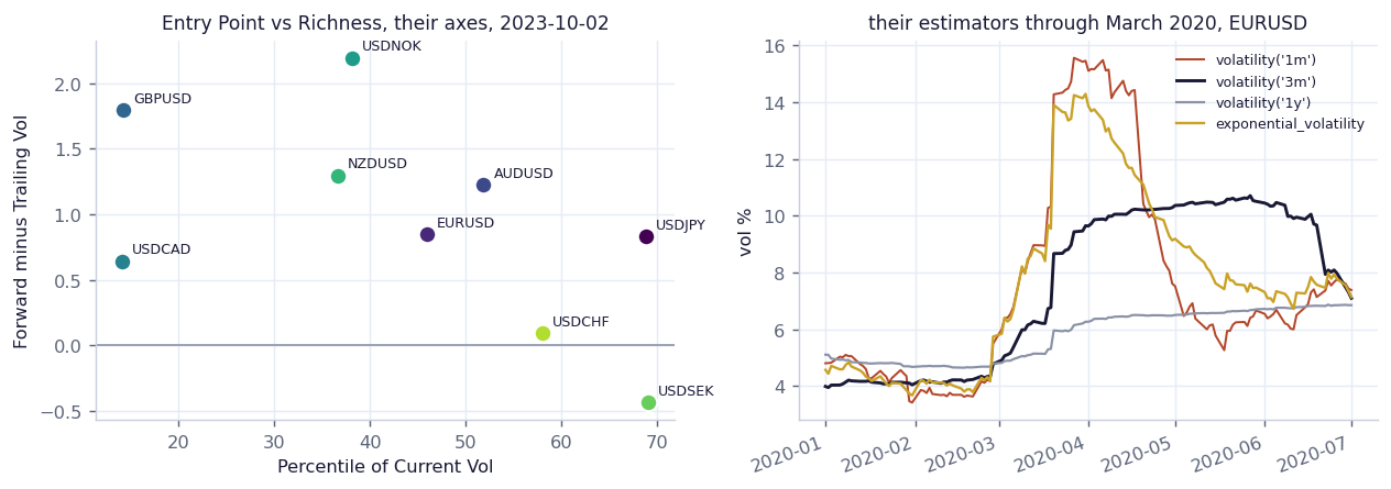
Left, their Entry Point vs Richness scatter on their axes. Right, their estimators through March 2020.
| Pair | Spot | 3m Realized | 3m Fwd Realized | Diff | %-ile |
|---|---|---|---|---|---|
| GBPUSD | 1.22 | 8.28 | 6.48 | +1.80 | 14.3 |
| USDCAD | 1.36 | 5.61 | 4.96 | +0.64 | 14.1 |
| NZDUSD | 0.60 | 10.24 | 8.94 | +1.30 | 36.6 |
| USDNOK | 10.68 | 13.32 | 11.12 | +2.19 | 38.2 |
| AUDUSD | 0.64 | 10.69 | 9.46 | +1.23 | 51.9 |
| USDCHF | 0.92 | 6.83 | 6.74 | +0.09 | 58.1 |
| USDSEK | 10.92 | 10.69 | 11.12 | -0.44 | 69.1 |
Screens like this exist because volatility mean reverts, so a low percentile is meant to mark a cheap entry. That is a testable claim and the repo gives you everything needed to test it.
pool = []
for c in G10:
    f = pd.DataFrame({"p": percentiles(spd[c]),      # their percentiles, expanding history
                      "d": diff[c]}).dropna()        # forward minus trailing vol
    pool.append(f)
    print(c, f.p.corr(f.d).round(3))

al = pd.concat(pool)
for lo, hi in [(0,20), (20,40), (40,60), (60,80), (80,101)]:
    s = al[(al.p >= lo) & (al.p < hi)]
print(f"{lo:3d}-{hi:3d} n={len(s):6,} {s.d.mean():+.2f} vol points")| Entry percentile | Observations | Volatility over the next 3 months |
|---|---|---|
| bottom quintile | 2,657 | +1.52 |
| 2nd | 2,002 | +0.54 |
| middle | 1,966 | +0.48 |
| 4th | 2,274 | -0.44 |
| top quintile | 4,016 | -1.25 |
Monotone across all five buckets, with a spread of 2.77 volatility points between the cheapest and the most expensive entry. It holds pair by pair too, with the correlation between entry percentile and subsequent change running from -0.296 on USDSEK to -0.510 on USDCAD, negative on all nine, pooled at -0.376. Screen is measuring something real.
One caveat their code carries and does not flag. percentiles(x) with no window ranks against an ever growing history rather than a fixed lookback, so the 2018 observations are ranked against a few months of data and the 2023 ones against six years. It is backward looking, so there is no lookahead, but the early percentiles are noisier than the late ones. Passing Window(504, 0) fixes it and weakens the pooled correlation to roughly -0.3, which is still the same conclusion.
What this does not tell you is whether the trade makes money, because that needs the option price and the option price needs Marquee. Volatility rising 1.52 points after a cheap entry is worth nothing if the option already charged you two points for the privilege. It is a tilt on which pair to express a view in, not a reason to have the view.
Since all of them run offline, they can be put on the same series and compared directly. EURUSD, 2018 to 2023:
| Estimator | Mean | Std dev | Min | Max | March 2020 peak |
|---|---|---|---|---|---|
volatility('1m') | 6.88 | 2.39 | 2.89 | 15.56 | 15.56 |
volatility('3m') | 6.97 | 2.03 | 3.86 | 12.59 | 10.71 |
volatility('6m') | 7.02 | 1.79 | 4.34 | 11.19 | 8.14 |
volatility('1y') | 7.10 | 1.47 | 4.65 | 10.03 | 6.72 |
exponential_volatility(0.94) | 6.94 | 2.20 | 3.42 | 14.55 | 14.29 |
vol_swap_volatility | 7.26, a single number for the whole sample rather than a series | ||||
They agree on the level, between 6.88 and 7.26, and disagree completely on the extremes. One month estimator peaked at 15.56 in March 2020 while the one year estimator peaked at 6.72, less than half. Both are correct. They answer different questions, and a risk limit written against one of them is a different limit from the same number written against another.
Correlation between the shortest and longest window is 0.446, which is the number to keep. Two estimators of the same quantity, on the same data, from the same library, agreeing less than half the time. Choosing the window is a bigger decision than choosing the library.
exponential_volatility correlates 0.966 with the one month window and reaches half of the March 2020 move two days sooner, so it behaves like a fast window without the cliff edge of one dropping out of a fixed lookback.
Their correlation and beta take any two series, so the screen's machinery transfers straight to equities and bonds. Same calls, different inputs:
# pip install gs-quant yfinance pandas
import pandas as pd, yfinance as yf
import gs_quant.timeseries as ts
from gs_quant.timeseries import Window

# ---------- data collection: free, no account ----------
px = yf.download(["SPY", "TLT"], start="2010-01-01", end="2024-01-01",
                 progress=False, auto_adjust=True)["Close"]
px = px.dropna(axis=1, thresh=250).ffill(limit=1).dropna(how="any")

out = pd.DataFrame(index=px.index)
out["vol_63"]  = ts.volatility(px.SPY, "3m")
out["corr_63"] = ts.correlation(px.SPY, px.TLT, Window(63, 0))
out["beta_63"] = ts.beta(px.SPY, px.TLT, Window(63, 0))
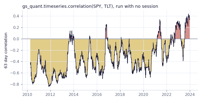
Gold is the hedge working, stocks and bonds moving apart. Red is the hedge failing.
| Period | Mean correlation | Days negative |
|---|---|---|
| 2010 to 2020 | -0.426 | 95% |
| 2022 onward | +0.060 | 44% |
For a decade the correlation was negative on 95% of days, which is the assumption the 60/40 portfolio rests on. From 2022 it averages plus 0.060 and is negative less than half the time. Both legs fell together in 2022 and that is why the year hurt as much as it did.
Correlation belongs in a volatility page because it is the second half of portfolio variance:
σ2p = w2Aσ2A + w2Bσ2B + 2 wA wB ρ σA σB
That last term flips sign with rho. Moving rho from minus 0.426 to plus 0.060 raises portfolio volatility without a single component becoming more volatile.
Of 48 timeseries functions tested, 46 ran with no session. Two that did not are excess_returns and sharpe_ratio, and they fail for the same reason: both need a risk free rate curve, which they fetch from Marquee by get_marquee_id. Substituting a free rate series and calling the pure form underneath, excess_returns_pure, works.
Their pricing engine, gs_quant.instrument and gs_quant.markets, is genuinely gated, as is every implied volatility surface. That is the boundary: their analytics are yours, their data is not.
If you have never fitted a volatility model, run the arch script first. It needs nothing but an internet connection, it finishes in seconds, and the persistence number it prints will change how you think about selling premium after a spike.
Then jump to SVI. Between those two you have a forecast of realised volatility and a clean read on implied volatility, which is both halves of the only trade that matters here: is the insurance too expensive or too cheap.
QuantLib and FinancePy are what you reach for once you want to know why the smile has the shape it does and what your position is actually exposed to. tf-quant-finance matters when calibration gets slow, which happens sooner than you expect. gs-quant sits last because it is the one where free data buys you the least, and it is worth reading rather than running.
Data behind all of this: four free sources for historical option chains
The greeks these models produce: vanna, volga, color, zomma and speed
I post the models as I build them, the changes I make to them, and the results that did not work. Shorter than these write ups, and there are a lot more of them.
Follow me on X