
Data from OpenBB, a screen from a TradingView MCP server, prices from QuantLib, a second opinion from TradingAgents, backtests from vectorbt, and orders to an Interactive Brokers paper account. One integration step for each, and the loop that joins them.
Whatever drives a strategy, it runs the same steps: data in, a signal, a price for the instrument, a backtest, and an order out with the fill read back. Each tool below covers one of those steps, each is free at the point of use, and each section shows the single call that plugs it in. All scripts ran on 19 October 2026 except 2: TradingAgents needs an LLM and the Interactive Brokers engine needs TWS open, so those were checked against the installed libraries and the upstream source instead.

py -3 <file>.py, with a
README that lists what each one printed:
github.com/davidalmeida90/quant-models/tree/main/quant-options-tools
| Tool | Step | Free tier | Licence, stars |
|---|---|---|---|
| OpenBB | Data in: chains, macro, fundamentals | Cboe, yfinance, Federal Reserve data, no key | Apache 2.0, about 74,000 |
| TradingView MCP | Screen | No TradingView account or key | MIT, about 5,000 |
| QuantLib | Price | All of it | BSD style, about 7,700 |
| TradingAgents | Signal from an LLM committee | Code; LLM local or paid | Apache 2.0, about 112,000 |
| vectorbt | Backtest thousands of settings | Open source edition | Apache 2.0 with Commons Clause, about 9,400 |
| Interactive Brokers | Order out, paper account | Paper account with any IBKR login | ib_async: BSD 2, about 1,800 |
Star counts are rounded from GitHub on the day of the check and measure adoption, nothing more. vectorbt's Commons Clause allows using it to trade, and rules out selling the software or a service built mostly on it.
2 builds that run the last steps of this page for real. A gamma exposure bot reads the free Cboe chain and trades Micro E-mini S&P futures on an Interactive Brokers paper account. TradingAgents runs on DeepSeek, from setup to a broker order.
Models as they are built, the changes made to them, and the results that did not work. Shorter than these write ups, and many more of them.
Follow on X


OpenBB is an open data platform, Apache 2.0, about 74,000 stars. One Python object,
obb, fronts dozens of data providers and returns DataFrames, so a strategy reads
every source through the same kind of call. Version 5 groups the calls by provider: the SPY
chain is obb.cboe.options.chains, the yield curve is
obb.federal_reserve.treasury_rates. Cboe, the Federal Reserve, SEC and FRED come
with pip install openbb; yfinance is one more package, openbb-yfinance.
For an options strategy that means the full chain with implied vol and Greeks on every strike and expiry, the underlying's price history, the VIX, Treasury yields and company metrics, with no key and no account.
File: openbb_data.py. It finds the expiry closest to 30 days, averages call and put implied vol at the strike closest to spot, and sets it against 21 day realized vol from daily closes.
from datetime import date, timedelta

import numpy as np
from openbb import obb

SYMBOL = "SPY"
since = (date.today() - timedelta(days=90)).isoformat()

# 1. option chain: every listed expiry and strike, with implied vol and Greeks
chain = obb.cboe.options.chains(SYMBOL).to_df()
spot = float(chain["underlying_price"].iloc[0])
expiry = chain.loc[(chain["dte"] - 30).abs().idxmin(), "expiration"]          # expiry closest to 30 days
month = chain[chain["expiration"] == expiry]
atm = month.loc[(month["strike"] - spot).abs().idxmin(), "strike"]
iv30 = month.loc[month["strike"] == atm, "implied_volatility"].mean()          # call and put at the money

# 2. realized vol over 21 trading days, annualized
close = obb.yfinance.equity.price.historical(SYMBOL, start_date=since).to_df()["close"]
rv21 = np.log(close).diff().tail(21).std() * np.sqrt(252)

# 3. macro: VIX and the 10 year Treasury yield
vix = obb.yfinance.index.price.historical("^VIX", start_date=since).to_df()["close"].iloc[-1]
ust10 = obb.federal_reserve.treasury_rates(start_date=since).to_df()["year_10"].iloc[-1]

# 4. fundamentals, for a single stock strategy
nvda = obb.yfinance.equity.fundamental.metrics("NVDA").to_df().iloc[0]

print(f"{SYMBOL} {spot:.2f}, {len(chain):,} contracts, expiry {expiry} "
      f"({int(month['dte'].iloc[0])} days), ATM strike {atm:g}")
print(f"implied vol 30d {iv30:.1%}, realized vol 21d {rv21:.1%}, ratio {iv30 / rv21:.2f}")
print(f"VIX {vix:.2f}, 10 year Treasury {ust10:.2%}")
print(f"NVDA forward P/E {nvda['forward_pe']:.1f}, operating margin {nvda['operating_margin']:.1%}")

# signal input: options rich against realized vol favour selling premium, cheap favour buying it
# (1.2 and 0.8 are placeholders, set them from your own backtest)
ratio = iv30 / rv21
print("IV/RV signal:", "sell premium" if ratio > 1.2 else "buy premium" if ratio < 0.8 else "no edge")| Field | Value | Source |
|---|---|---|
| SPY, contracts in the chain | 767.35, 12,730 | Cboe |
| Expiry used, days | 20 Nov 2026, 32 | Cboe |
| At the money implied vol, 30 days | 14.1% | Cboe, strike 767 |
| Realized vol, 21 days | 10.2% | yfinance closes |
| Implied over realized | 1.38 | computed |
| VIX | 18.65 | yfinance |
| 10 year Treasury | 5.10% | Federal Reserve |
| NVDA forward P/E, operating margin | 13.5, 66.2% | yfinance |
Implied vol at 14.1% against 10.2% realized puts the ratio at 1.38: SPY options were priced rich to how much the index had actually moved. A premium selling strategy reads that as its entry condition. Cut offs of 1.2 and 0.8 in the script are placeholders, to be set from a backtest. VIX sits above the at the money vol because it also prices the out of the money puts and their skew.
An MCP server exposes functions to an AI client over the Model Context Protocol. This one, by atilaahmettaner, MIT, about 5,000 stars, wraps TradingView's screener and technical analysis data, plus Yahoo prices, into 37 tools: gainers and losers, Bollinger scans, multi timeframe analysis, option chains and backtests. No TradingView account or key.
Inside Claude or Cursor it answers in a chat. Inside a strategy the same tools work as a screen:
a Python MCP client starts the server, calls a tool and gets JSON back. Below, 6 Nasdaq names
go through coin_analysis on the daily timeframe (the name says coin, it covers
stocks too), and only names in an uptrend that are not overbought stay on the watchlist.
File: tradingview_mcp_client.py. uvx runs the server from PyPI in its own environment, as the server's README installs it.
import asyncio
import json

from mcp import ClientSession, StdioServerParameters
from mcp.client.stdio import stdio_client

SERVER = StdioServerParameters(command="uvx", args=["--from", "tradingview-mcp-server", "tradingview-mcp"])
WATCHLIST = ["AAPL", "MSFT", "NVDA", "AMZN", "META", "TSLA"]


async def call(tv, tool, **args):
    res = await tv.call_tool(tool, args)
    return [json.loads(c.text) for c in res.content]          # one JSON block per row


async def main():
    async with stdio_client(SERVER) as (read, write), ClientSession(read, write) as tv:
        await tv.initialize()
        print(len((await tv.list_tools()).tools), "tools on the server")
        keep = []
        for sym in WATCHLIST:
            await asyncio.sleep(2)                                    # TradingView throttles bursts of calls
            a = (await call(tv, "coin_analysis", symbol=sym, exchange="NASDAQ", timeframe="1D"))[0]
            if "error" in a:                                          # TradingView throttles, skip and move on
                err = a["error"]
                print(f"{sym:<5} skipped, {err.get('code', '') if isinstance(err, dict) else err}")
                continue
            close, sma200, rsi = a["price_data"]["close"], a["sma"]["sma200"], a["rsi"]["value"]
            bb = a["market_sentiment"]["overall_rating"]           # Bollinger position, -3 to +3
            ok = close > sma200 and rsi < 70 and bb >= 0              # uptrend, not overbought, upper half
            print(f"{sym:<5} close {close:>8.2f}  SMA200 {sma200:>8.2f}  RSI {rsi:5.1f}  BB {bb:+d}  "
                  f"{'keep' if ok else 'skip'}")
            keep.append(sym) if ok else None
        print("watchlist for the strategy:", keep)


asyncio.run(main())
Run on 19 October 2026, the server started and listed 37 tools, then TradingView's scanner
answered every analysis call with UPSTREAM_ERROR for several minutes, a throttle
after a burst of test calls. A single call an hour earlier had gone through: AAPL closed at
343.46, above its 200 day average of 292.46, RSI 62.1, Bollinger rating +2, which passes the
filter. Hence the 2 second pause between symbols, and the skip on error instead of a crash.
One install trap. A plain pip install tradingview-mcp-server on Python 3.14 falls
back to version 0.7.1, because 0.8.x declares Python below 3.14, and 0.7.1 imports a module
that mcp 2.x removed. uvx resolves 0.8.1 with mcp 1.x and works. Registering it in Claude Code
is one line: claude mcp add tradingview -- uvx --from tradingview-mcp-server tradingview-mcp.
QuantLib is an open source C++ library for pricing and risk on derivatives and fixed income,
with Python bindings on PyPI (pip install QuantLib). BSD style licence, about 7,700
stars. Its Examples/EquityOption file prices one put with European, Bermudan and
American exercise using 21 methods, from Black-Scholes and Heston to binomial trees, finite
differences and Longstaff Schwartz Monte Carlo.
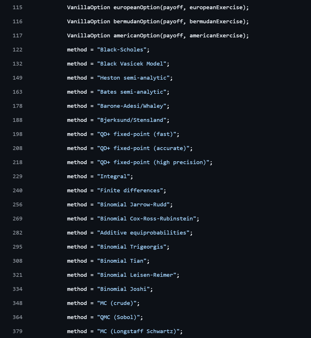
File: quantlib_pricing.py. Same inputs as the C++ file: spot 36, strike 40, rate 6%, vol 20%, 1 year. 20 of the 21 run in Python; Black Vasicek has no binding in QuantLib 1.44.
methods = [   # (name, engine, which exercise styles it prices)
    ("Black-Scholes", ql.AnalyticEuropeanEngine(bsm), E),
    # Black Vasicek, method 2 of the C++ file, has no Python binding in QuantLib 1.44, so 20 of 21 here
    ("Heston semi-analytic", ql.AnalyticHestonEngine(heston), E),
    ("Bates semi-analytic", ql.BatesEngine(bates), E),
    ("Barone-Adesi/Whaley", ql.BaroneAdesiWhaleyApproximationEngine(bsm), A),
    ("Bjerksund/Stensland", ql.BjerksundStenslandApproximationEngine(bsm), A),
    ("QD+ fixed-point (fast)", qdfp(bsm, qdfp.fastScheme()), A),
    ("QD+ fixed-point (accurate)", qdfp(bsm, qdfp.accurateScheme()), A),
    ("QD+ fixed-point (high precision)", qdfp(bsm, qdfp.highPrecisionScheme()), A),
    ("Integral", ql.IntegralEngine(bsm), E),
    ("Finite differences", ql.FdBlackScholesVanillaEngine(bsm, steps, steps - 1), ALL),
] + [(name, ql.BinomialVanillaEngine(bsm, tree, steps), ALL) for name, tree in [| Method | European | Bermudan | American |
|---|---|---|---|
| Black-Scholes | 3.844308 | ||
| Heston semi-analytic | 3.844306 | ||
| Bates semi-analytic | 3.844306 | ||
| Barone-Adesi/Whaley | 4.459628 | ||
| Bjerksund/Stensland | 4.453064 | ||
| QD+ fixed-point (fast) | 4.486617 | ||
| QD+ fixed-point (accurate) | 4.486669 | ||
| QD+ fixed-point (high precision) | 4.486674 | ||
| Integral | 3.844309 | ||
| Finite differences | 3.844330 | 4.360765 | 4.486113 |
| Binomial Jarrow-Rudd | 3.844132 | 4.361174 | 4.486552 |
| Binomial Cox-Ross-Rubinstein | 3.843504 | 4.360861 | 4.486415 |
| Additive equiprobabilities | 3.836911 | 4.354455 | 4.480097 |
| Binomial Trigeorgis | 3.843557 | 4.360909 | 4.486461 |
| Binomial Tian | 3.844171 | 4.361176 | 4.486413 |
| Binomial Leisen-Reimer | 3.844308 | 4.360713 | 4.486076 |
| Binomial Joshi | 3.844308 | 4.360713 | 4.486076 |
| MC (crude) | 3.834522 | ||
| QMC (Sobol) | 3.844613 | ||
| MC (Longstaff Schwartz) | 4.456935 |
On the European put, analytic, tree, lattice and simulation methods agree on 3.844 to the third decimal, crude Monte Carlo aside. American exercise adds about 0.64 of early exercise value, 4.4867 on the precise methods. Barone-Adesi/Whaley and Bjerksund/Stensland are fast closed form approximations and land 2.7 and 3.4 cents low, the trade a strategy makes when it reprices a whole chain every few seconds. Whole script runs in 0.6 seconds.
What a strategy calls on every quote it reads. Feed it the bid or ask from the OpenBB chain and it gets its own implied vol and hedge ratios, independent of the vendor's Greeks.
def quote_to_greeks(price, spot, strike, days, rate, div=0.0, right=ql.Option.Put):
    """Implied vol from a quoted European price, then delta, gamma, vega at that vol."""
    expiry = today + ql.Period(days, ql.Days)
    vol_q = ql.SimpleQuote(0.20)
    proc = ql.BlackScholesMertonProcess(
        ql.QuoteHandle(ql.SimpleQuote(spot)),
        ql.YieldTermStructureHandle(ql.FlatForward(today, div, dc)),
        ql.YieldTermStructureHandle(ql.FlatForward(today, rate, dc)),
        ql.BlackVolTermStructureHandle(ql.BlackConstantVol(today, cal, ql.QuoteHandle(vol_q), dc)))
    opt = ql.VanillaOption(ql.PlainVanillaPayoff(right, strike), ql.EuropeanExercise(expiry))
    opt.setPricingEngine(ql.AnalyticEuropeanEngine(proc))
    vol_q.setValue(opt.impliedVolatility(price, proc))
    return {"iv": vol_q.value(), "delta": opt.delta(), "gamma": opt.gamma(), "vega": opt.vega() / 100}


print("\nquote 4.00 on the same put:", {k: round(v, 4) for k, v in quote_to_greeks(4.00, 36, 40, 365, 0.06).items()})
A quote of 4.00 on the same put implies 21.09% vol, delta of minus 0.544, gamma 0.052 and vega 0.143 per vol point. Above the model's 3.844 at 20%, so the market price carries about 1.1 vol points more than the model assumes.
github.com/lballabio/QuantLib · Examples/EquityOption/EquityOption.cpp
TradingAgents by Tauric Research is a multi agent LLM framework that runs a trading firm in miniature: 4 analysts, a bull and a bear researcher, a trader, a risk team and a portfolio manager. Apache 2.0, about 112,000 stars, paper arXiv 2412.20138. Its output is one of 5 ratings, Buy, Overweight, Hold, Underweight or Sell, with the reasoning behind it.
Every agent is an LLM call, so a run costs API credit or local compute. Through Ollama it runs
on a local model for free; on DeepSeek a full run costs about 6 cents. For a strategy, the
rating becomes a side: Buy and Overweight map to BUY, Underweight and Sell to SELL, Hold to no
trade, and a REVIEW (no readable rating) never trades. Paired with the price the committee saw,
it returns the same (side, reference_price) pair the router at the end of this page
expects, so the committee can stand in for any other signal or veto it.
File: tradingagents_signal.py.
Local model by default (ollama pull qwen3:8b); TA_PROVIDER=deepseek
with DEEPSEEK_API_KEY in the environment switches to DeepSeek.
import os
import sys
from datetime import date

import yfinance as yf
from tradingagents.default_config import DEFAULT_CONFIG
from tradingagents.graph.trading_graph import TradingAgentsGraph

# Buy, Overweight, Hold, Underweight, Sell; REVIEW (no readable rating) is not in the map, so no trade
SIDE = {"Buy": "BUY", "Overweight": "BUY", "Hold": None, "Underweight": "SELL", "Sell": "SELL"}


def tradingagents_signal(symbol, trade_date=None, provider=os.environ.get("TA_PROVIDER", "ollama")):
    config = DEFAULT_CONFIG.copy()
    config["max_debate_rounds"] = 1
    if provider == "ollama":                              # local model, free, through Ollama on port 11434
        config["llm_provider"] = "ollama"
        config["backend_url"] = "http://localhost:11434/v1"
        config["deep_think_llm"] = config["quick_think_llm"] = "qwen3:8b"
    else:                                                 # DeepSeek, about 6 cents a full run
        config["llm_provider"] = "deepseek"
        config["deep_think_llm"], config["quick_think_llm"] = "deepseek-v4-pro", "deepseek-v4-flash"
    ta = TradingAgentsGraph(debug=False, config=config)
    _, rating = ta.propagate(symbol, trade_date or date.today().isoformat())
    ref = float(yf.Ticker(symbol).history(period="5d")["Close"].iloc[-1])    # price the committee saw
    return SIDE.get(rating), ref


if __name__ == "__main__":
    sym = sys.argv[1] if len(sys.argv) > 1 else "NVDA"
    print(sym, tradingagents_signal(sym))                # ('BUY', last close), or (None, last close) on Hold
Not run for this page, since it needs an LLM. Its calls were checked against the TradingAgents
source on 19 October 2026: propagate returns the final state and the rating, and
the 5 tier scale with the REVIEW fallback lives in tradingagents/agents/rating.py.
Second video above runs the whole committee on DeepSeek, debate included.
vectorbt runs backtests as arrays. Every parameter set becomes a column and numba compiles the loops, so a grid of thousands of settings runs as one vectorized call on pandas and NumPy. Apache 2.0 with Commons Clause, about 9,400 stars.
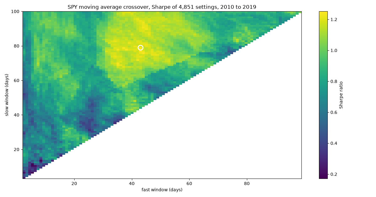
Here it sweeps every fast and slow moving average pair from 2 to 100 days on SPY, 4,851 settings, over 2010 to 2019 with 5 basis points a trade. Best pair by Sharpe then runs on 2020 onward, data the sweep never saw, next to buy and hold.
File: vectorbt_sweep.py. A warm up on a small slice compiles numba first, so the printed time is the backtest itself.
px = yf.download("SPY", start="2010-01-01", auto_adjust=True, progress=False)["Close"]["SPY"]
ins, oos = px[:"2019-12-31"], px["2020-01-01":]

warm = ins.iloc[:200]                    # compile numba once on a small slice, so the timing below is the backtest
wf, ws = vbt.MA.run_combs(warm, window=[2, 3, 4], r=2)
vbt.Portfolio.from_signals(warm, wf.ma_crossed_above(ws), wf.ma_crossed_below(ws), freq="1D").sharpe_ratio()

# 1. all 4,851 pairs at once, fast window below slow window, 5 bp a trade
t0 = time.perf_counter()
fast, slow = vbt.MA.run_combs(ins, window=np.arange(2, 101), r=2, short_names=["fast", "slow"])
entries, exits = fast.ma_crossed_above(slow), fast.ma_crossed_below(slow)
pf = vbt.Portfolio.from_signals(ins, entries, exits, fees=0.0005, freq="1D")
sharpe = pf.sharpe_ratio()
secs = time.perf_counter() - t0
print(f"{sharpe.size:,} backtests on {len(ins):,} days in {secs:.1f} s")

# 2. best pair in sample, then the same pair out of sample against buy and hold
f, s = sharpe.idxmax()
print(f"in sample  2010-2019: best fast {f}, slow {s}, Sharpe {sharpe.max():.2f}, "
      f"median of all {sharpe.median():.2f}, buy and hold {vbt.Portfolio.from_holding(ins, freq='1D').sharpe_ratio():.2f}")
mf, ms = vbt.MA.run(px, f), vbt.MA.run(px, s)                     # full history so the windows are warm on day 1
oos_pf = vbt.Portfolio.from_signals(oos, mf.ma_crossed_above(ms)[oos.index], mf.ma_crossed_below(ms)[oos.index],
                                    fees=0.0005, freq="1D")
hold = vbt.Portfolio.from_holding(oos, freq="1D")
print(f"out of sample {oos.index[0]:%Y}-{oos.index[-1]:%Y}: pair {f}/{s} Sharpe {oos_pf.sharpe_ratio():.2f}, "
      f"return {oos_pf.total_return():.0%}, max drawdown {oos_pf.max_drawdown():.0%} | "
      f"buy and hold Sharpe {hold.sharpe_ratio():.2f}, return {hold.total_return():.0%}, "
f"max drawdown {hold.max_drawdown():.0%}")| Period, setting | Sharpe | Return | Max drawdown |
|---|---|---|---|
| 2010 to 2019, best of 4,851 (43/79) | 1.25 | ||
| 2010 to 2019, median setting | 0.88 | ||
| 2010 to 2019, buy and hold | 1.11 | ||
| 2020 to 2026, 43/79 | 1.08 | 101% | −21% |
| 2020 to 2026, buy and hold | 0.96 | 158% | −34% |
4,851 backtests on 2,516 trading days took 2.2 seconds, after about 19 seconds of one time numba compile. A Sharpe of 1.25 picked from 4,851 tries fell to 1.08 on data the sweep never saw. Out of sample it still beat buy and hold on Sharpe and drawdown by sitting out part of the falls, and made 101% against 158%. Choosing the best of thousands flatters the winner, which is why the second half of the data stays locked until the pair is picked.
Every Interactive Brokers account comes with a paper account, a username starting with DU, and the same API as live. TWS or IB Gateway runs on the desktop and the API is a socket on localhost: port 7497 for TWS paper, 4002 for Gateway paper. ib_async, BSD 2, about 1,800 stars, is the maintained Python client.
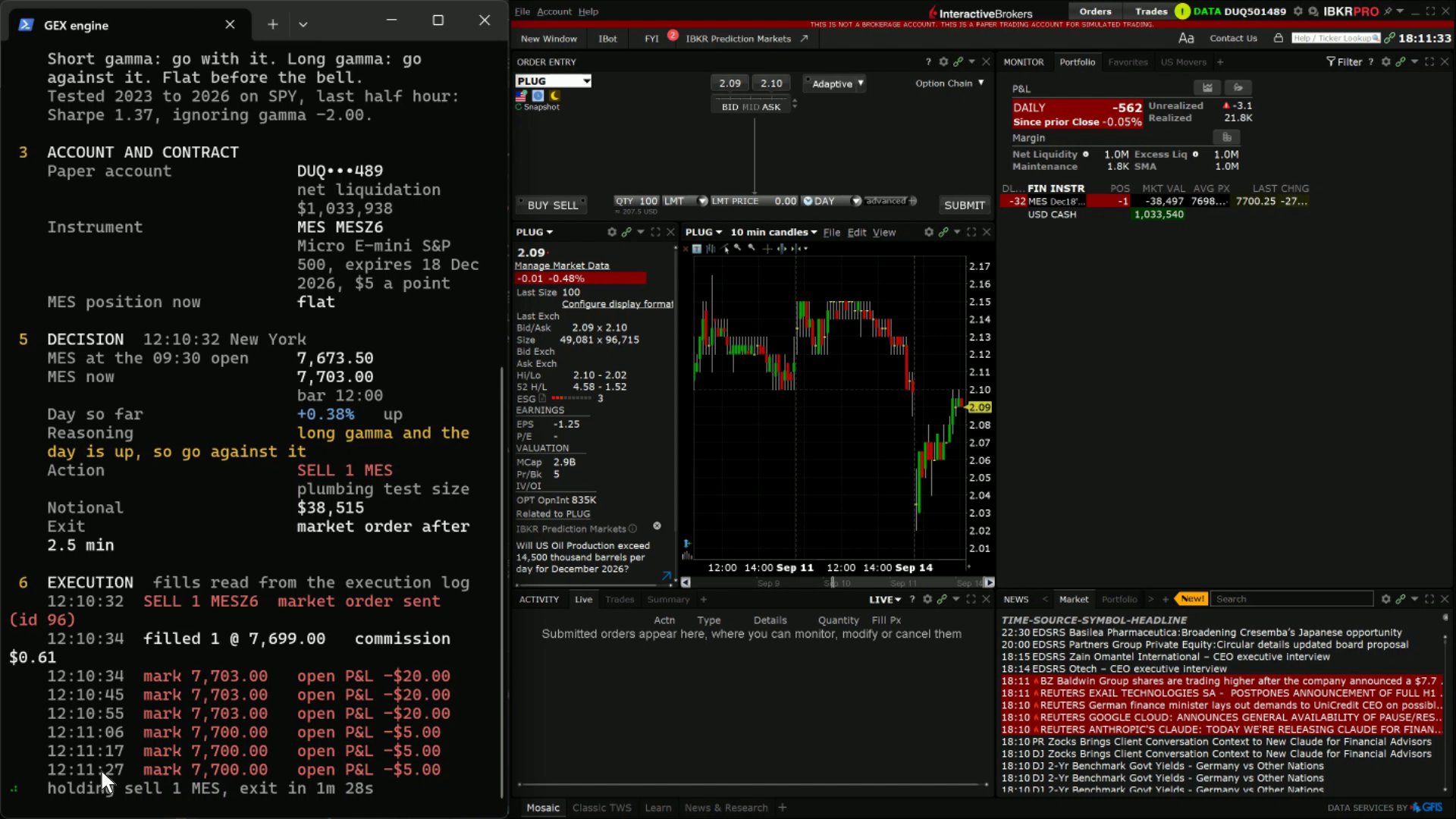
This step turns a backtest into orders. ibkr_engine.py refuses anything but a paper
port and a DU account, picks a contract (a SPY share, or a SPY put about 30 days out and 5%
below spot from the chain IBKR lists), sends a market or limit order, and reads the fill back
from the executions.
File: ibkr_engine.py.
py -3 ibkr_engine.py buys 1 SPY share; --put 2.50 buys 1 SPY put at a
2.50 limit instead.
PAPER_PORTS = (7497, 4002)                         # TWS paper, IB Gateway paper; live ports are refused


def connect(port=7497, client_id=11):
    if port not in PAPER_PORTS:
        raise SystemExit(f"port {port} is not a paper port")
    ib = IB()
    ib.connect("127.0.0.1", port, clientId=client_id)
    if not ib.managedAccounts()[0].startswith("DU"):           # paper account ids start with DU
        ib.disconnect()
        raise SystemExit("not a paper account")
return ibdef send(ib, contract, side, qty, limit=None, wait_s=10):
"""Place the order, wait on executed quantity, return the average fill price (None if unfilled)."""
trade = ib.placeOrder(contract, LimitOrder(side, qty, limit) if limit else MarketOrder(side, qty))
for _ in range(wait_s * 2): # wait on fills, not on isDone(): a parent order can
if trade.filled() >= qty: # report Cancelled while its executions are correct
break
ib.sleep(0.5)
done = sum(f.execution.shares for f in trade.fills)
return sum(f.execution.shares * f.execution.price for f in trade.fills) / done if done else NoneNot run for this page: it needs TWS logged into a paper account. Every ib_async call in it was checked against version 2.1.0. Two TWS settings decide whether it works at all, both under Global Configuration, API, Settings: tick Enable ActiveX and Socket Clients, untick Read-Only API. With Read-Only on, account reads work and every order comes back rejected.
Fills come from the executions. A parent order can report Cancelled while its child executions are correct, so the wait loop keys on executed quantity, never on the order status.
interactivebrokers.com › TWS · github.com/ib-api-reloaded/ib_async
One file runs the whole chain. loop.py reads SPY, applies the 43 and 79 day rule
vectorbt picked, backtests it, routes the order with the skeleton from
trading-integration/route.py,
and reads the fill back. Any step can take the tool above it: OpenBB for the data, the
TradingView screen for the symbol list, tradingagents_signal as the signal, a
QuantLib price as the limit on an option order.
ibkr_engine.py.
File: loop.py.
--broker dry (default) fills at the last close so it runs anywhere;
--broker ibkr sends a real paper order.
def route(signal_fn, symbol="SPY", qty=QTY, broker="dry", max_notional=50_000, log=LOG):
    side, ref = signal_fn(symbol)                                       # 4. route, skeleton of route.py
    if side is None or qty * ref > max_notional:                        # risk check before any broker call
        return None
    if broker == "ibkr":
        from ib_async import Stock
        from ibkr_engine import connect, send
        ib = connect()
        contract = Stock(symbol, "SMART", "USD")
        ib.qualifyContracts(contract)
        fill = send(ib, contract, side, qty)                            # 5. fill, read from the executions
        ib.disconnect()
    else:
        fill = ref                                                      # dry run: fill at the reference price
    row = {"t": datetime.now(timezone.utc).isoformat(timespec="seconds"), "broker": broker, "symbol": symbol,
           "side": side, "qty": qty, "signal_px": round(ref, 2), "fill_px": fill and round(fill, 2),
           "slip_bps": fill and round(1e4 * (fill - ref) / ref, 1)}     # signed, compare with the backtest weekly
    os.makedirs(os.path.dirname(log), exist_ok=True)
    with open(log, "a") as f:
        f.write(json.dumps(row) + "\n")
    return row


if __name__ == "__main__":
    ap = argparse.ArgumentParser()
    ap.add_argument("--broker", default="dry", choices=["dry", "ibkr"])
    broker = ap.parse_args().broker

    px = data("SPY")
    long = rule(px)
    pf = backtest(px, long)
    print(f"backtest {px.index[0]:%Y-%m-%d} to {px.index[-1]:%Y-%m-%d}: Sharpe {pf.sharpe_ratio():.2f}, "
          f"return {pf.total_return():.0%}, max drawdown {pf.max_drawdown():.0%}, {pf.trades.count()} trades")

    def ma_signal(symbol):                                              # target today minus what is held
        gap = (QTY if long.iloc[-1] else 0) - held(symbol, broker)
        return ("BUY" if gap > 0 else "SELL" if gap < 0 else None), float(px.iloc[-1])

    print(f"rule on {px.index[-1]:%Y-%m-%d}: {'long' if long.iloc[-1] else 'flat'} ({FAST}/{SLOW} day MA)")
print("order:", route(ma_signal, broker=broker))backtest 2015-01-02 to 2026-10-16: Sharpe 0.64, return 104%, max drawdown -32%, 13 trades
rule on 2026-10-16: long (43/79 day MA)
order: {'t': '2026-10-19T11:31:34+00:00', 'broker': 'dry', 'symbol': 'SPY', 'side': 'BUY', 'qty': 10, 'signal_px': 763.25, 'fill_px': 763.25, 'slip_bps': 0.0}
Dry run on 19 October 2026: the rule was long on the 16 October close and nothing was held, so
it routed BUY 10 SPY at 763.25. A second run read the position back from the log and sent
nothing. With --broker ibkr the same lines reach TWS paper and the slippage column
starts to carry information. Compared weekly with the backtest's fill assumption, the gap is
what latency, spread and data cost the strategy.
Free trading tools covers Alpaca, Glassbench and QuantConnect Lean, with the first version of the routing skeleton. Free options data covers where chains come from. Gamma exposure is the strategy behind the first video, and time series momentum runs a larger parameter sweep with the same in sample, out of sample discipline.