
One trend following rule, 990 versions of it, on 45 free ETFs from 2005 to 2026. Lookback crossed against holding period, scored on the first decade and then checked on the second, with the published grid from Moskowitz, Ooi and Pedersen beside it.
Most published backtests show one equity curve and one set of parameters. What they do not show is the other 989 versions that were tried and discarded, and that omission is where a great many disappointing live results come from.
This page runs the search in the open. A trend following rule from a well known 2012 paper is rebuilt on free data, every parameter combination is scored, the single best one is picked exactly the way anyone would pick it, and then it is dropped onto a decade that played no part in choosing it. Full Python, every chart, every table, and an audit that tries to break the thing on purpose.
Nothing here is a recommendation and nothing here is tradeable as written. It is a worked example of how far a result travels once you stop grading it on the data that produced it.
I build quantitative finance models on camera and publish the code here. Option pricing and the Greeks, volatility surfaces, asset allocation, and lately how far agentic AI can be pushed on real investment work. Every video has a page like this one behind it, with the script and the numbers, so nothing has to be taken on trust.
I post the models as I build them, the changes I make to them, and the results that did not work. Shorter than these write ups, and there are a lot more of them.
Follow me on X


One trend following rule, 990 versions of it, run end to end on real prices. Time series momentum says an instrument's own past return predicts its own next return. Two numbers decide how that rule behaves: how far back you look, and how long you hold what you decide. Everything below sweeps both across a grid, scores every setting, and then checks how much survives on a decade the search was never allowed to see.
Data is 45 liquid ETFs spanning equity indices, bonds, commodities, currencies and real assets. Adjusted daily closes from Yahoo, 3 January 2005 to 14 August 2026, 5,438 trading days. Costs are charged on every position change. Nothing is simulated and no seed stands in for a result.
Two claims get tested. First, whether a published result reproduces at all on data the authors never touched. Second, and more useful, what a parameter search does to you when you let it look 990 times at the same decade.
Read the limitations before trusting any number here. ETFs stand in for futures, the sample overlaps the original paper by five years at most, and the split is one date rather than a rolling walk forward.
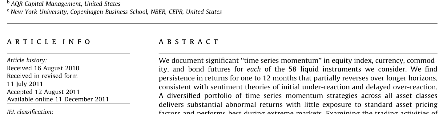
Moskowitz, Ooi and Pedersen, Time Series Momentum, Journal of Financial Economics 104(2), 2012. Their claim is narrow and testable, which is exactly what makes it worth rebuilding. Worth reading in their own words first.
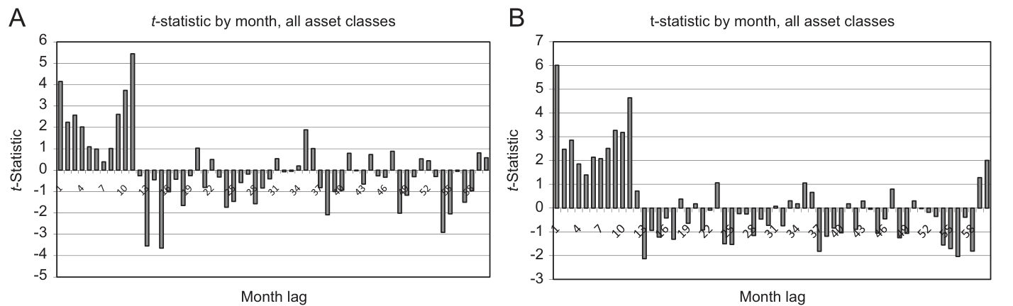
Their Figure 1 is the evidence behind that sentence. Each contract's monthly excess return is regressed on its own lagged return at every horizon from one month out to 60, pooled across all 58 instruments, with standard errors clustered by month. Bars are t-statistics.
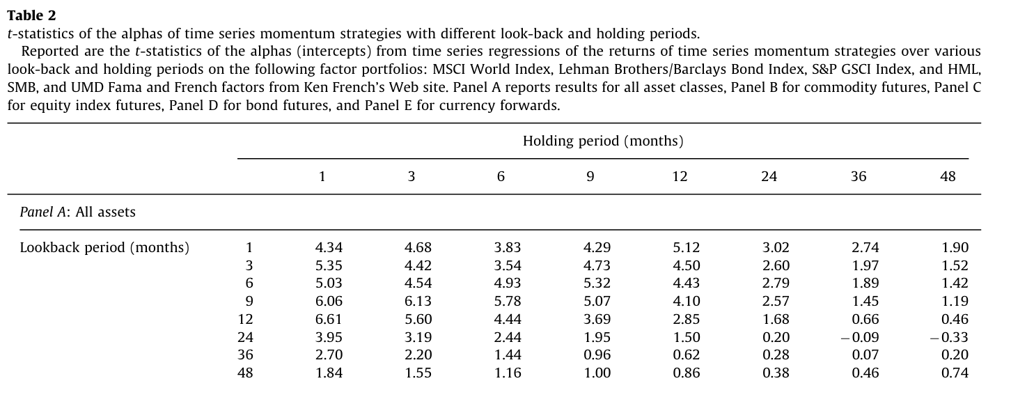
Their Table 2 is the part this page rebuilds directly. Lookback period is crossed against holding period and the t-statistic of the alpha is reported in every cell, after controlling for the equity market, bonds, commodities and the three Fama and French factors. Eight values on each axis, 64 cells.
Grid built below is that table at higher resolution: 33 lookbacks against 30 holding periods instead of 8 by 8, on daily data rather than monthly, on ETFs rather than futures, over a sample that begins roughly where theirs ends. Shape is what gets compared. Never the level.
Four libraries, all free. No data subscription is used anywhere on this page, and the same script runs on a laptop in about two minutes.
Shell
pip install yfinance pandas numpy pyarrow matplotlibPaper uses 58 futures contracts, which cost money to obtain. Closest free stand in is a basket of liquid ETFs covering the same four asset classes, plus a small real assets sleeve. Adjusted closes handle dividends and splits. Pull once, cache to parquet, and never touch the network again, so every rerun is reproducible.
Python
import numpy as np, pandas as pd, yfinance as yf
import matplotlib.pyplot as plt

ETFS = [
    ## equity indices, 17 names, developed and emerging
    "SPY","QQQ","IWM","DIA","MDY","EFA","EEM","EWJ","EWG","EWU",
    "EWZ","EWY","EWA","EWC","FXI","EWH","EWW",
    ## government, corporate, high yield and inflation linked bonds
    "TLT","IEF","SHY","LQD","HYG","TIP","AGG","BWX","EMB",
    ## commodities, energy through to precious metals and agriculture
    "GLD","SLV","USO","UNG","DBA","DBB","DBC","DBO","PPLT",
    ## developed market currencies against the dollar
    "FXE","FXY","FXB","FXA","FXF","FXC","UUP",
    ## real assets
    "IYR","VNQ","XLE",
]

raw = yf.download(ETFS, start="2005-01-01", auto_adjust=True, progress=False)
px  = raw["Close"].dropna(how="all").ffill(limit=3)   ## bridge up to 3 stale days
px.to_parquet("etfs.parquet")

print(f"{px.shape[0]:,} days x {px.shape[1]} names")
print(f"{px.index[0].date()} to {px.index[-1].date()}")
## 5,438 days x 45 names
## 2005-01-03 to 2026-08-14| Asset class | ETFs | Members |
|---|---|---|
| Equity indices | 17 | SPY, QQQ, IWM, DIA, MDY, EFA, EEM, EWJ, EWG, EWU, EWZ, EWY, EWA, EWC, FXI, EWH, EWW |
| Bonds | 9 | TLT, IEF, SHY, LQD, HYG, TIP, AGG, BWX, EMB |
| Commodities | 9 | GLD, SLV, USO, UNG, DBA, DBB, DBC, DBO, PPLT |
| Currencies | 7 | FXE, FXY, FXB, FXA, FXF, FXC, UUP |
| Real assets | 3 | IYR, VNQ, XLE |
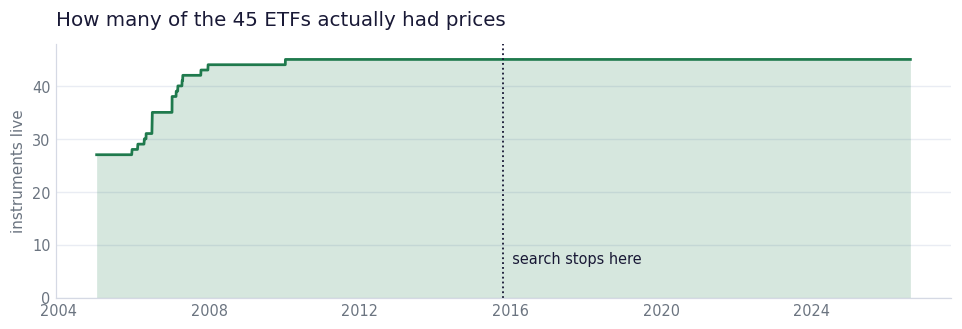
Not all 45 exist from day one. Several launched during the sample, so the panel widens over time and the early years run on a thinner basket. That is handled by masking rather than by dropping, so no instrument contributes a return on a day it did not trade.
Signal is the sign of the return over the last L days. Nothing more. If price
today sits above where it was L days ago, go long, otherwise go short. Magnitude
is thrown away on purpose, which matches the paper's sign specification in their Panel B and
stops one violent instrument from dominating the book.
L is the lookback window, swept over 33 values from 5 to 300
trading days. Spacing is logarithmic, so the short end gets the resolution it needs while the
long end still reaches beyond a year.
Python
## 33 lookbacks x 30 holdings = 990 complete backtests
LOOKBACK = np.unique(np.round(np.logspace(np.log10(5), np.log10(300), 34)).astype(int))
HOLDING  = np.unique(np.round(np.logspace(np.log10(1), np.log10(250), 36)).astype(int))

live = px.notna()                    ## True only where the ETF actually traded
R    = px.pct_change().fillna(0.0)

def signal(L):
    """+1 if it rose over the last L days, -1 if it fell.

    px.shift(L) is the price L rows ago, so this only ever reads prices up to
    and including today. Nothing from the future enters here.
    """
    return np.sign(px / px.shift(L) - 1.0).fillna(0.0).where(live, 0.0)

print(LOOKBACK)
## [  5   6   7   8   9  11  12  14  16  18  21  24  27  31  36  41  47  54
##   62  71  81  93 107 122 140 160 184 210 241 276 300]
Holding a view for H days raises an awkward question: which day do you start? Pick
one and the whole result depends on an arbitrary calendar choice, and a strategy that changes
answer depending on whether you began on a Monday is not a strategy.
Fix used by the paper, and used here, is to run H books opened one day apart and
average them, so every possible start date is represented equally. Written out, that is
simply a rolling mean of the last H daily decisions. A position of +0.4 means
roughly 70% of the recent decisions said long.
Python
def held(L, H):
    """H overlapping books opened a day apart, averaged into one position.

    min_periods=H means no position at all until H days of signal exist, so
    the book does not quietly start trading on a half filled window.
    """
return signal(L).rolling(H, min_periods=H).mean().fillna(0.0)Each instrument is scaled to a 40% annualised volatility target using its own trailing 60 day realised volatility, capped at three times notional. That is the paper's construction, and it stops natural gas from swamping a short dated bond fund inside an equal weighted basket.
Volatility is measured on data up to and including today, and the resulting position earns tomorrow's return. Cost is 2 basis points of notional every time a position moves, charged on the absolute change, which is generous for liquid ETFs and brutal for the corner of the grid that wants to rebalance daily.
Python
COST, VOL_WIN, TARGET_VOL, CAP = 2e-4, 60, 0.40, 3.0

## ex ante volatility: uses returns through today, never beyond
vol   = (R.pow(2).rolling(VOL_WIN, min_periods=VOL_WIN).mean() * 252).pow(0.5)
scale = (TARGET_VOL / vol).clip(upper=CAP).fillna(0.0)

def backtest(L, H):
    """One complete backtest of the 45 name basket."""
    pos  = held(L, H) * scale
    ## pos.shift(1) is the whole no-look-ahead rule: position set at the close
    ## of day t earns the return of day t+1
    pnl  = pos.shift(1) * R - COST * (pos - pos.shift(1)).abs()
    turn = (pos - pos.shift(1)).abs().where(live)
    return (pnl.where(live).mean(axis=1).fillna(0.0),      ## equal weight
            float(turn.mean(axis=1).mean() * 252))          ## turnover per year
Cost assumption is doing more work than it looks. A one day holding period rebuilds the whole book every session, which at 2 basis points is a drag of over four percent a year before a single trend is caught.
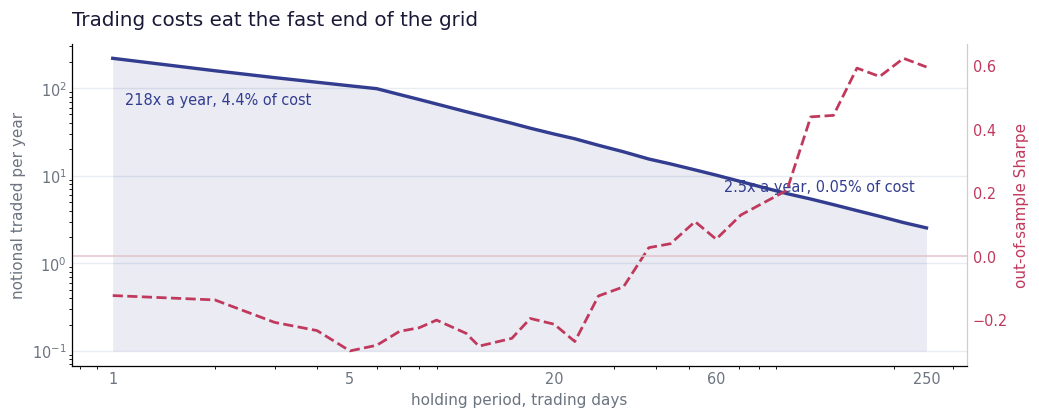
| Holding | Turnover per year | Cost drag | In-sample | Out-of-sample |
|---|---|---|---|---|
| 1 day | 218.7× | 4.37% | −0.61 | −0.12 |
| 5 days | 106.2× | 2.12% | −0.36 | −0.30 |
| 11 days | 53.8× | 1.08% | −0.11 | −0.24 |
| 23 days | 26.4× | 0.53% | +0.09 | −0.27 |
| 52 days | 11.6× | 0.23% | +0.40 | +0.11 |
| 83 days | 7.3× | 0.15% | +0.77 | +0.17 |
| 133 days | 4.7× | 0.09% | +0.51 | +0.44 |
| 250 days | 2.5× | 0.05% | +0.52 | +0.60 |
Sample splits in half at 21 October 2015, 2,719 trading days either side. First half is where the search is allowed to look. Second half is scored afterwards, using whichever setting the search chose, and is never consulted while choosing.
Python
SPLIT  = len(px) // 2                                  ## 2015-10-21
sharpe = lambda x: x.mean() / x.std(ddof=1) * np.sqrt(252)

ISR  = np.zeros((len(LOOKBACK), len(HOLDING)))         ## in sample
OOS  = np.zeros_like(ISR)                              ## out of sample
TURN = np.zeros_like(ISR)                              ## turnover per year

for a, L in enumerate(LOOKBACK):
    for b, H in enumerate(HOLDING):
        p, t = backtest(int(L), int(H))
        p = p.to_numpy()
        ISR[a, b]  = sharpe(p[:SPLIT])                 ## the search sees this
        OOS[a, b]  = sharpe(p[SPLIT:])                 ## and never this
        TURN[a, b] = t

## the search picks the single best in-sample cell, which is the whole point
BI, BJ = np.unravel_index(ISR.argmax(), ISR.shape)
print(f"winner: {LOOKBACK[BI]}d lookback held {HOLDING[BJ]}d")
print(f"  in  {ISR[BI, BJ]:+.3f}")
print(f"  out {OOS[BI, BJ]:+.3f}")
## winner: 6d lookback held 83d
##   in  +0.771
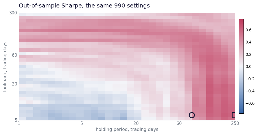
## out +0.169Every figure on this page comes out of the block below. Two heatmaps of the same grid, one per sample half, on a shared colour scale so they can be read against each other.
Python
## ---- the ten settings the search liked most, and what each did afterwards ----
top = np.argsort(ISR.ravel())[::-1][:10]
print(f"{'look':>5} {'hold':>5} {'in':>7} {'out':>7} {'kept':>6}")
for k in top:
    i, j = np.unravel_index(k, ISR.shape)
    print(f"{LOOKBACK[i]:5d} {HOLDING[j]:5d} {ISR[i,j]:+7.3f} {OOS[i,j]:+7.3f} "
          f"{OOS[i,j]/ISR[i,j]*100:5.0f}%")

## ---- the grid, twice, on one shared colour scale ----
lim = np.abs(np.r_[ISR.ravel(), OOS.ravel()]).max()
ext = (np.log10(HOLDING[0]), np.log10(HOLDING[-1]),
       np.log10(LOOKBACK[0]), np.log10(LOOKBACK[-1]))

for M, name, title in ((ISR, "grid_is.png",  "In-sample Sharpe, all 990 settings"),
                       (OOS, "grid_oos.png", "Out-of-sample Sharpe, the same 990")):
    fig, ax = plt.subplots(figsize=(10.5, 4.4))
    im = ax.imshow(M, aspect="auto", origin="lower", cmap="coolwarm",
                   vmin=-lim, vmax=lim, extent=ext)
    ## ring the cell the search chose, and square the slow one for comparison
    ax.scatter([np.log10(HOLDING[BJ])], [np.log10(LOOKBACK[BI])],
               s=140, facecolors="none", edgecolors="#191936", lw=2.0)
    ax.set_xticks(np.log10([1, 5, 20, 60, 250]))
    ax.set_xticklabels(["1", "5", "20", "60", "250"])
    ax.set_yticks(np.log10([5, 20, 60, 300]))
    ax.set_yticklabels(["5", "20", "60", "300"])
    ax.set_title(title, loc="left")
    ax.set_xlabel("holding period, trading days")
    ax.set_ylabel("lookback, trading days")
    fig.colorbar(im, ax=ax, pad=0.015, shrink=0.88)
    fig.savefig(name, dpi=110, bbox_inches="tight")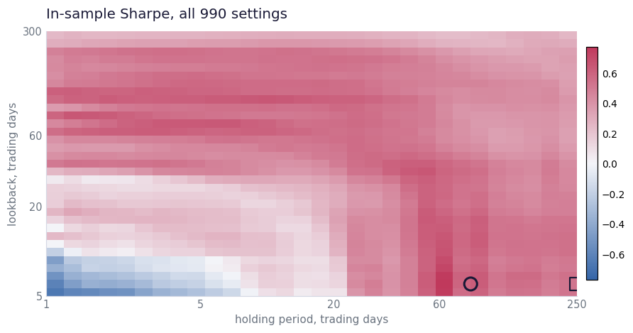
| Lookback | Holding | In-sample | Out-of-sample | Kept |
|---|---|---|---|---|
| 6 days | 83 days | +0.771 | +0.169 | 22% |
| 5 days | 83 days | +0.759 | +0.113 | 15% |
| 7 days | 83 days | +0.753 | +0.175 | 23% |
| 8 days | 83 days | +0.716 | +0.159 | 22% |
| 9 days | 83 days | +0.691 | +0.152 | 22% |
| 11 days | 83 days | +0.661 | +0.144 | 22% |
| 12 days | 83 days | +0.654 | +0.134 | 21% |
| 13 days | 83 days | +0.643 | +0.112 | 17% |
| 87 days | 2 days | +0.640 | +0.117 | 18% |
| 111 days | 17 days | +0.639 | +0.429 | 67% |
Nine of the top ten sit in the same vertical stripe at 83 days of holding, and all nine keep between 15% and 23% of what they promised. Tenth is different: a 111 day lookback held 17 days, almost as good in sample and it kept 67%. Search had no way to prefer it, because in sample it ranked tenth.
Heatmaps show where the good cells are. Slicing them says how fragile each one is, and that matters more.
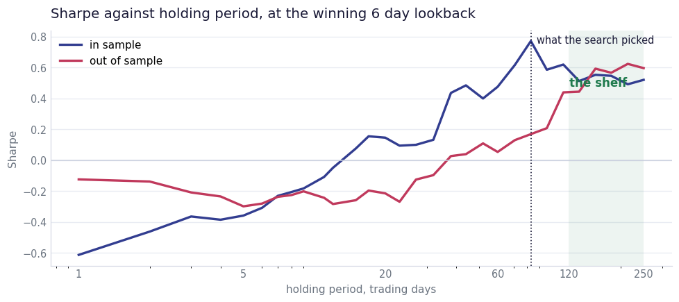
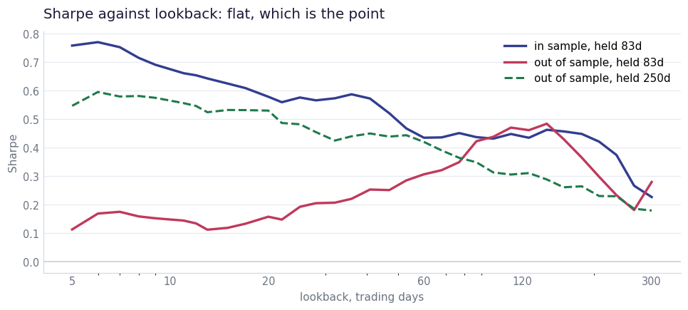
Asymmetry between those two charts is the practical finding on this page. One parameter barely matters and the other decides everything, and a grid search treats both as equally important because it has no way to know the difference.
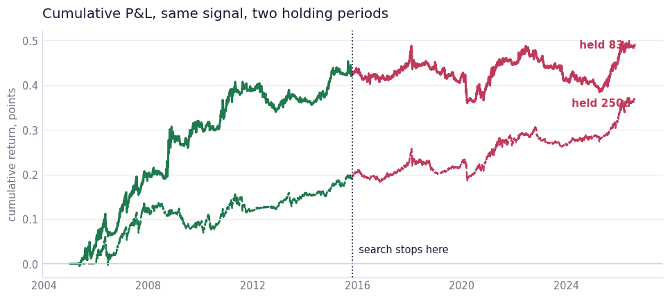
Search picks a 6 day lookback held 83 days, in-sample Sharpe +0.77. Same rule on the decade it never saw returns +0.17. Roughly three quarters of the in-sample figure was the search rewarding itself for looking 990 times at one decade.
| Book | Period | Cumulative | Per year | Volatility | Sharpe | Max drawdown |
|---|---|---|---|---|---|---|
| Held 83 days | in-sample | +42.4 pts | +3.93% | 5.1% | +0.77 | −6.8 |
| Held 83 days | out-of-sample | +6.6 pts | +0.61% | 3.6% | +0.17 | −12.8 |
| Held 250 days | in-sample | +19.3 pts | +1.79% | 3.4% | +0.52 | −6.7 |
| Held 250 days | out-of-sample | +17.8 pts | +1.65% | 2.8% | +0.60 | −7.3 |
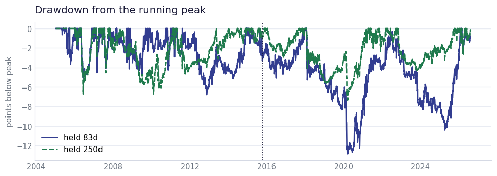
Worst drawdown on the fast book arrives after the split, at 12.8 points against 6.8 before it, so the setting the search liked delivered a fifth of the return with roughly twice the pain. Slow book barely notices the split at all.
| Year | Held 83d | Held 250d | Sample |
|---|---|---|---|
| 2005 | +4.0 | −0.1 | in |
| 2006 | +8.9 | +6.7 | in |
| 2007 | +7.0 | +5.7 | in |
| 2008 | +8.2 | −1.1 | in |
| 2009 | +2.7 | −2.3 | in |
| 2010 | +5.4 | +3.4 | in |
| 2011 | +2.9 | −0.4 | in |
| 2012 | −4.0 | +1.2 | in |
| 2013 | +2.0 | +2.7 | in |
| 2014 | +4.7 | +1.0 | in |
| 2015 | +1.3 | +3.6 | split |
| 2016 | −1.3 | −1.7 | out |
| 2017 | +3.6 | +4.4 | out |
| 2018 | −1.0 | −2.7 | out |
| 2019 | −2.4 | +2.2 | out |
| 2020 | −1.5 | +1.6 | out |
| 2021 | +4.3 | +3.8 | out |
| 2022 | +0.7 | +0.3 | out |
| 2023 | −4.0 | −1.4 | out |
| 2024 | −0.5 | +1.4 | out |
| 2025 | +4.5 | +4.2 | out |
| 2026 | +3.4 | +4.6 | out |
2008 is where the fast book earns its in-sample record, at +8.2 points while the slow one loses 1.1. Trend following is supposed to do exactly that in a crash. Out of sample it never gets another 2008, and six up years against five down years nearly cancel.
Level degrades, which is expected. What matters more is whether the map holds. Across all 990 cells the correlation between in-sample and out-of-sample Sharpe is +0.68, and 78% of the grid is still positive out of sample. On an overfit strategy that correlation sits near zero and the second heatmap goes cold everywhere.
Running the same comparison instrument by instrument gives the degradation line directly. Each ETF gets its own best setting chosen in sample, and is then scored out of sample with that same setting.
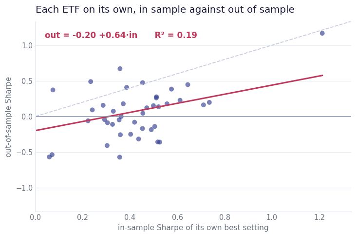
Slope of 0.77 says an extra point of in-sample Sharpe on an instrument bought 0.77 of a point out of sample, which is a genuinely steep slope. Intercept of −0.45 says every instrument gives back about that much simply for leaving the sample. Both effects are real and they work against each other, and the intercept is the one people forget.
Basket beats most of its own legs, and the reason is correlation rather than skill. Average pairwise correlation between the 45 individual momentum books is +0.18, which buys roughly a 2.2 times reduction in risk for the same return.
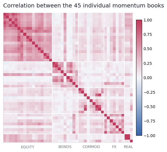
| Sleeve | Within | Against others |
|---|---|---|
| Equity indices | +0.47 | +0.13 |
| Bonds | +0.33 | +0.08 |
| Commodities | +0.25 | +0.10 |
| Currencies | +0.33 | +0.12 |
| Real assets | +0.39 | +0.15 |
| All 990 pairs | +0.18 |
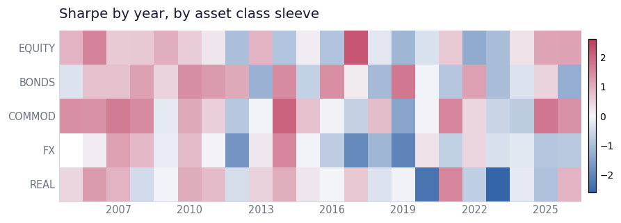
| Sleeve | ETFs | In-sample | Out-of-sample |
|---|---|---|---|
| Commodities | 9 | +0.85 | +0.49 |
| Bonds | 9 | +0.67 | +0.28 |
| Real assets | 3 | +0.53 | −0.22 |
| Equity indices | 17 | +0.48 | +0.07 |
| Currencies | 7 | +0.39 | −0.49 |
Commodities carry the book on both halves, which lines up with the paper reporting its strongest single asset class results there. Currencies go from +0.39 to −0.49, and since currency trend is the sleeve most often cited as having decayed since the crisis, that is at least a familiar failure rather than a surprising one.
Paper reports t-statistics of alphas. This reports Sharpe ratios of raw returns, on different instruments over a different period, so the two are not directly comparable in level. Shape is comparable, and shape is the interesting part. Below is this grid collapsed to the same horizons the paper uses, in months.
| Lookback | 1m | 3m | 6m | 9m | 12m |
|---|---|---|---|---|---|
| 1 month | +0.16 | +0.51 | +0.49 | +0.45 | +0.48 |
| 3 months | +0.51 | +0.51 | +0.34 | +0.38 | +0.35 |
| 6 months | +0.55 | +0.48 | +0.43 | +0.42 | +0.37 |
| 9 months | +0.52 | +0.48 | +0.38 | +0.36 | +0.34 |
| 12 months | +0.38 | +0.32 | +0.25 | +0.30 | +0.30 |
| Lookback | 1m | 3m | 6m | 9m | 12m |
|---|---|---|---|---|---|
| 1 month | +0.02 | +0.06 | +0.45 | +0.56 | +0.53 |
| 3 months | +0.17 | +0.16 | +0.54 | +0.54 | +0.42 |
| 6 months | +0.32 | +0.42 | +0.49 | +0.36 | +0.31 |
| 9 months | +0.39 | +0.39 | +0.27 | +0.24 | +0.26 |
| 12 months | +0.22 | +0.15 | +0.29 | +0.25 | +0.19 |
Every one of those 25 cells is positive on both halves, which is a stronger statement than anything the search produced. Best out-of-sample cell in the whole comparison is a 1 month lookback held 9 months at +0.56, more than three times what the search's pick delivered.
Grid stops at 12 months on both axes, so the reversal region the paper finds beyond month 13 is outside what these ETFs and this sample can reach. That part is untested here rather than contradicted.
Three structural rules, then four tests built to fail loudly if any of them leaked.
Signal uses prices up to today. Position formed at the close of day t
earns the return of day t+1, which is exactly what pos.shift(1)
does above.
Volatility sizing is ex ante. Trailing 60 day realised volatility through day
t, applied to that same position, scoring the next day.
Split is chronological. Winner is chosen on the first half alone, and the second half is never read while choosing.
Structure can be argued about, so each rule was attacked as well. Every test below is built so that a leak would show up as a large positive number.
Python
def audit(lag=1, vol_lag=0, sig_shift=0):
    """Rerun the winning cell with one guard deliberately broken."""
    sig = np.sign(px.shift(sig_shift) / px.shift(6 + sig_shift) - 1.0)
    sig = sig.fillna(0.0).where(live, 0.0)
    v   = (R.pow(2).rolling(60, min_periods=60).mean() * 252).pow(0.5)
    if vol_lag:
        v = v.shift(vol_lag)                       ## sizing cannot see today
    pos = sig.rolling(83, min_periods=83).mean().fillna(0.0) \
          * (0.40 / v).clip(upper=3.0).fillna(0.0)
    pnl = pos.shift(lag) * R - 2e-4 * (pos - pos.shift(1)).abs()
    return pnl.where(live).mean(axis=1).fillna(0.0).to_numpy()

base = audit()
print(f"honest              {sharpe(base[:SPLIT]):+.2f}")
print(f"same-day fill       {sharpe(audit(lag=0)[:SPLIT]):+.2f}")     ## cheating
print(f"signal sees +1 day  {sharpe(audit(sig_shift=-1)[:SPLIT]):+.2f}")  ## cheating
print(f"vol lagged a day    {sharpe(audit(vol_lag=1)[:SPLIT]):+.2f}")
## honest              +0.77
## same-day fill       +1.21
## signal sees +1 day  +1.15
## vol lagged a day +0.76| Test | In-sample Sharpe | Reading |
|---|---|---|
| Reported backtest | +0.77 | baseline |
| Fill on the same day the signal is formed | +1.21 | hindsight is worth +0.44, and is not taken |
| Let the signal see tomorrow's price | +1.15 | another +0.38 on offer, not taken |
| Lag the volatility estimate one extra day | +0.76 | unchanged, so sizing carries no future |
| Execute two days late instead of one | +0.77 | no collapse, nothing depended on the edge |
| Execute five days late | +0.70 | gentle decay, the signature of a slow signal |
Last two rows carry most of the weight. Look-ahead collapses the moment lag is added, because the information it was stealing is one day old and gone. A genuine trend signal decays gently, which is what happens here: out-of-sample Sharpe moves from +0.17 to +0.16 to +0.17 across one, three and five days of extra delay.
Different data from the paper, and that is the big one. Moskowitz, Ooi and Pedersen use 58 futures contracts from 1985 to 2009. This uses 45 ETFs from 2005 to 2026. Overlap is five years at most, several holdings are close substitutes for one another, with SPY and DIA and MDY the obvious case, and an ETF carries a management fee and a tracking difference that a futures contract does not. Any comparison to their t-statistics is a comparison of shapes, never of levels.
Grid does not reach their horizons. Holding tops out at 250 trading days, roughly 12 months, and lookback at 300 days. Reversal region the paper documents beyond month 13 sits outside this grid entirely, so nothing here confirms or contradicts it.
Costs are one flat number. Two basis points on every position change, with no spread widening in a crisis, no market impact, and no short borrow charge. Short end of the holding axis suffers most from this being wrong, and it is already the weakest region.
One split, not a walk forward. Everything rests on a single date, 21 October 2015. A rolling walk forward would give many out-of-sample windows instead of one, and is the honest next step for anyone wanting to trade this rather than read about it.
Panel is not constant. Roughly 30 of the 45 ETFs exist in 2005 and all 45 by about 2010, so the in-sample half runs on a narrower and differently composed basket than the out-of-sample half. Some of the degradation between halves is that, and separating the two would need a fixed universe.
Return levels are arbitrary. Each instrument is targeted at 40% volatility and then 45 of them are equal weighted, which drags portfolio volatility to roughly 5%. Cash figures in the tables above are a consequence of that scaling choice. Only the Sharpe ratios compare to anything.
Survivorship, mildly. ETF list is today's liquid names, so funds that closed over the period are absent. Effect is far smaller than it would be on single stocks, and it is not zero.
Out-of-sample has now been looked at. Once results from the second half are read and discussed, as they are on this page, that half stops being a clean holdout for any future decision. Numbers here describe what happened. They do not forecast.
Machine learning for equity and fixed income reproduces a different published paper on free data and runs into the same wall from the other side. Five machine learning papers that reshaped quant finance is the reading list behind both. Volatility convexity with straddles and strangles builds a position rather than a signal.