Options models for fixed income

1. Callable and puttable bonds

A callable bond lets the issuer buy it back, usually at par after a few years of call protection, so the holder is short a call. When rates fall the issuer refinances and the bond is called away, so its price stalls near the call price: negative convexity. A puttable lets the holder sell it back at par, and that put sets a floor under the price when rates rise.

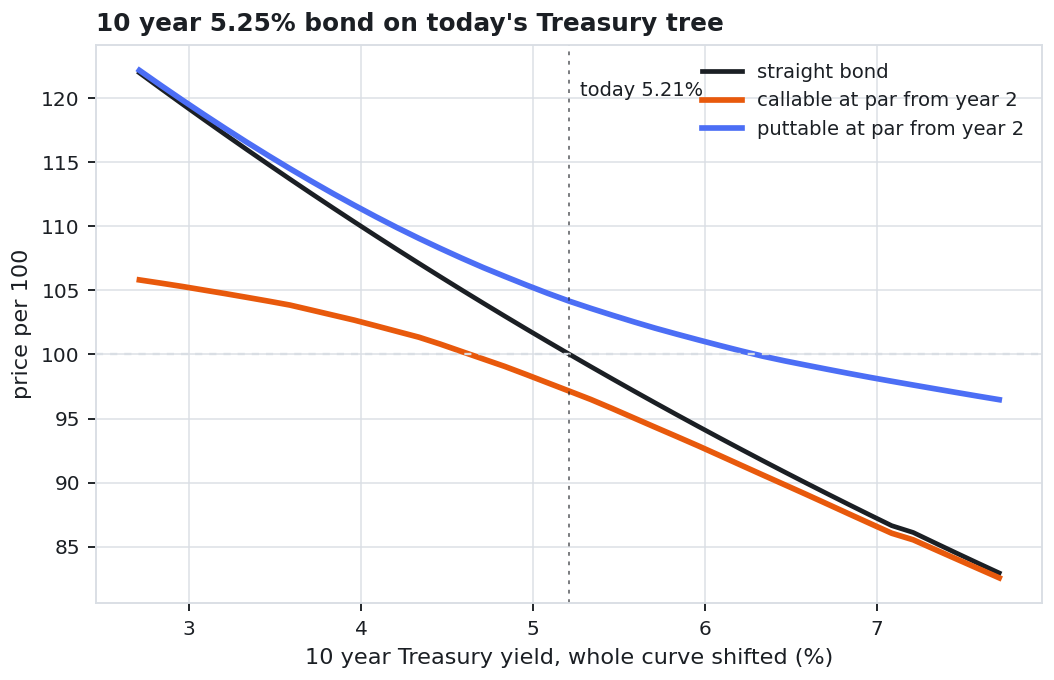
A Black-Derman-Toy tree reprices every discount factor of the 2026-10-13 curve, with a rate vol of 14% measured from one year of the 1 year yield. Stepping back from maturity and exercising wherever it pays puts the issuer's call at 2.88 per 100 and the holder's put at 4.14.

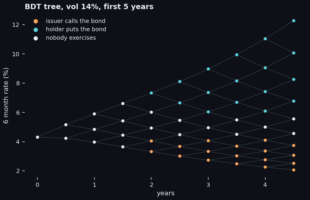
Pricing a callable or puttable bond on the tree

def bond_price(R, dt, T, coupon, kind="straight", K=100.0, first=2.0, freq=2):
    """Backward induction on the BDT short rate tree R. "call": the issuer calls
    at K on any coupon date from year `first`; "put": the holder puts at K."""
    n, step, c = int(round(T / dt)), int(round(1 / (freq * dt))), 100 * coupon / freq
    V = np.full(n + 1, 100.0 + c)
    for i in range(n - 1, -1, -1):
        V = np.exp(-R[i, :i + 1] * dt) * 0.5 * (V[1:i + 2] + V[:i + 1])
        if i > 0 and i % step == 0:
            if i * dt >= first:
                V = np.minimum(V, K) if kind == "call" else np.maximum(V, K) if kind == "put" else V
            V = V + c
    return float(V[0])

2. Convertible bonds

A convertible is a bond the holder can swap for a fixed number of shares, so it sits on two floors: the bond and the stock. Tsiveriotis and Fernandes (1998) split its value on a stock tree. Cash the bond still owes is discounted with credit risk, and the part that ends up as shares is discounted risk free.

Take UBER at $71.32, one year realised vol of 35%, and a hypothetical 5 year 1% convertible that converts 30% above today's price. With cash discounted at Treasuries plus the 1.03% ICE BofA BBB spread, the bond alone is worth 78.4 and the shares 76.9. On the tree the convertible is worth 102.6, so the right to convert adds 24.1.

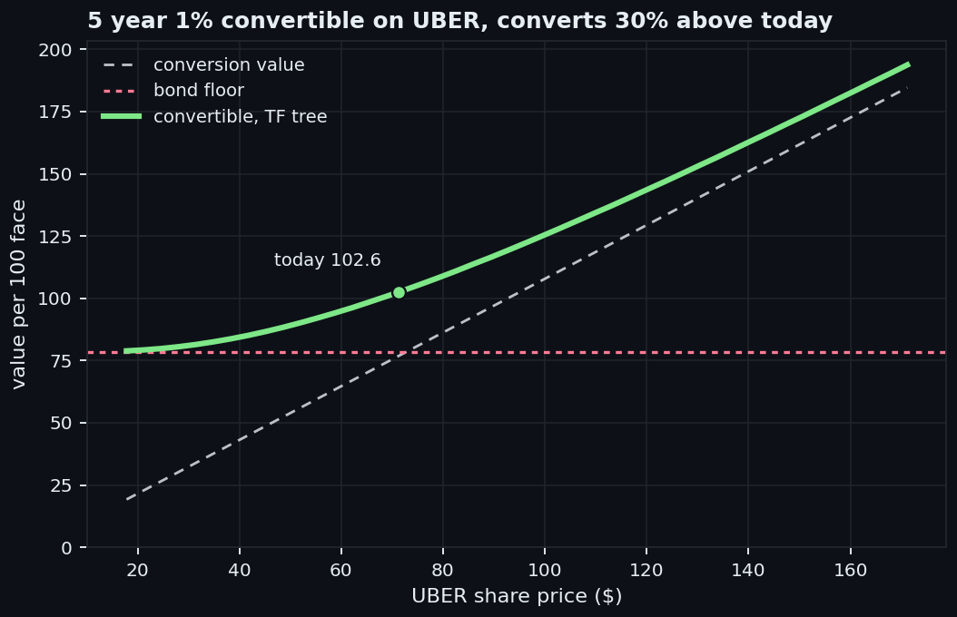
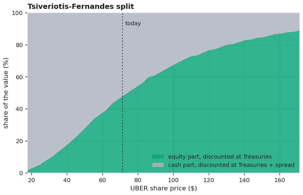
Tsiveriotis-Fernandes, backward through the stock tree

for i in range(n - 1, -1, -1):
    S = S[:-1] / u
    B = np.exp(-(r + spread) * dt) * (p * B[:-1] + (1 - p) * B[1:])   # credit risky
    E = np.exp(-r * dt) * (p * E[:-1] + (1 - p) * E[1:])              # risk free
    if i > 0 and i % step == 0:
        B = B + coupon
    convert = CR * S > B + E
    E = np.where(convert, CR * S, E)
    B = np.where(convert, 0.0, B)
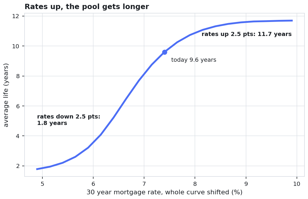
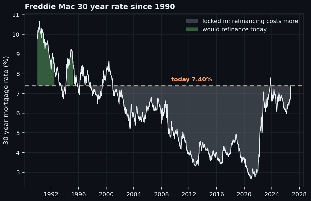
price = B[0] + E[0]

3. Mortgage-backed security prepayment option

A US mortgage can be repaid at par any day with no penalty, so every homeowner holds a call: when rates fall, they refinance. A mortgage-backed security pools thousands of these loans, and its holder is short all those calls. Prices stop rising when rates fall, and the bond gets longer when they rise.

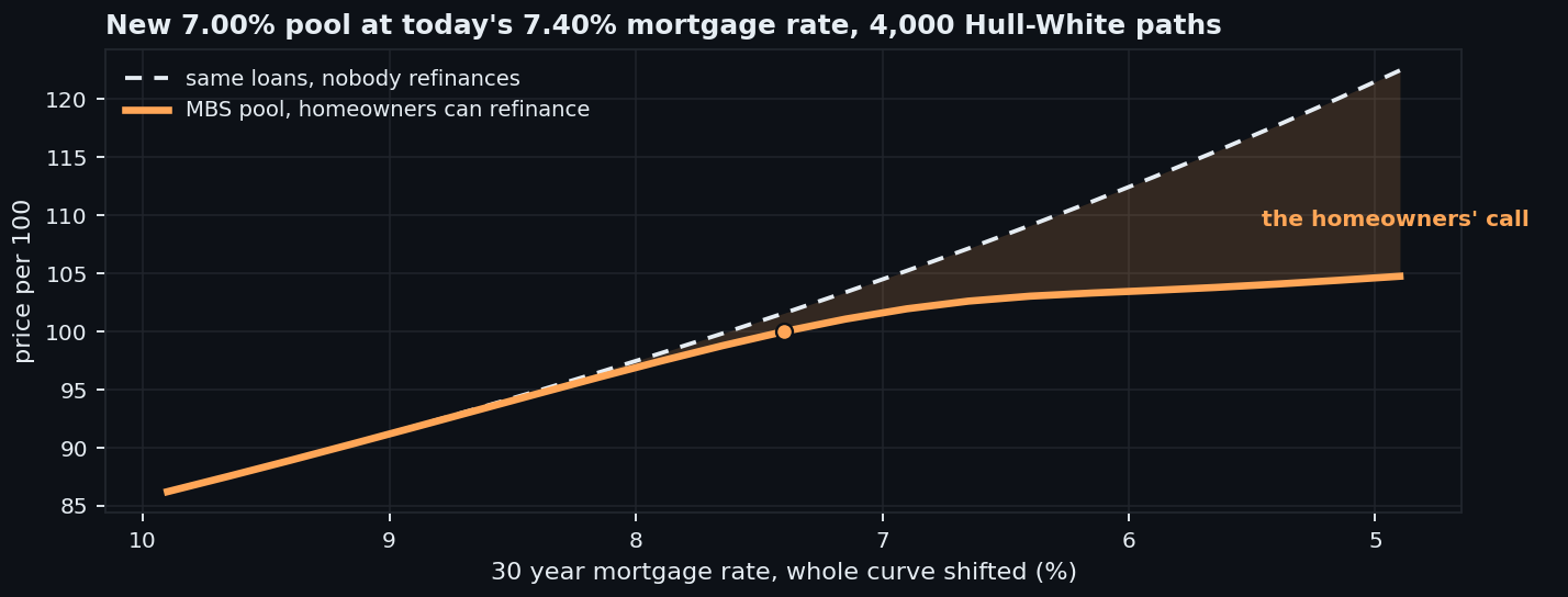
Rates come from Hull-White paths with the vol set so the 10 year yield moves 67 bp a year, as it did over the last year, and a simple S-curve decides who refinances. If rates fall 1 point, the pool gains 3.1, against 7.6 for the same loans if nobody could refinance. If they rise 1 point, it loses 5.4.

Pool cash flows on each rate path, with the refinancing S-curve

for k in range(360):
    sched = bal * w / (1 - (1 + w) ** -(360 - k)) - bal * w       # scheduled principal
    cpr = 0.06 * min(1.0, (k + 1) / 30)                            # housing turnover
    cpr = cpr + 0.45 / (1 + np.exp(-((wac - m[:, k]) - 0.01) / 0.002))   # refinancing
    prep = (1 - (1 - cpr) ** (1 / 12)) * (bal - sched)
    cf[:, k] = bal * coupon / 12 + sched + prep
    bal = bal - sched - prep

price = (cf * disc * np.exp(-oas * t)).sum(1).mean()               # average over the paths

4. Merton credit model

Merton showed in 1974 that a company's shares are a call option on its assets, struck at what it owes. If the assets end below the debt, shareholders walk away and lenders take the firm. So a corporate bond is a safe bond minus a put on the company. Moody's EDF default model grew out of this idea.

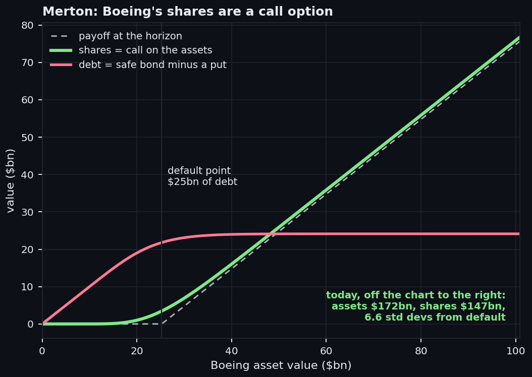
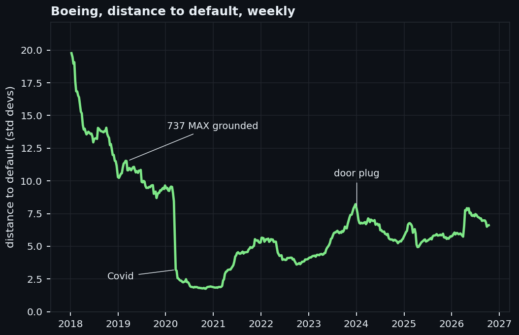
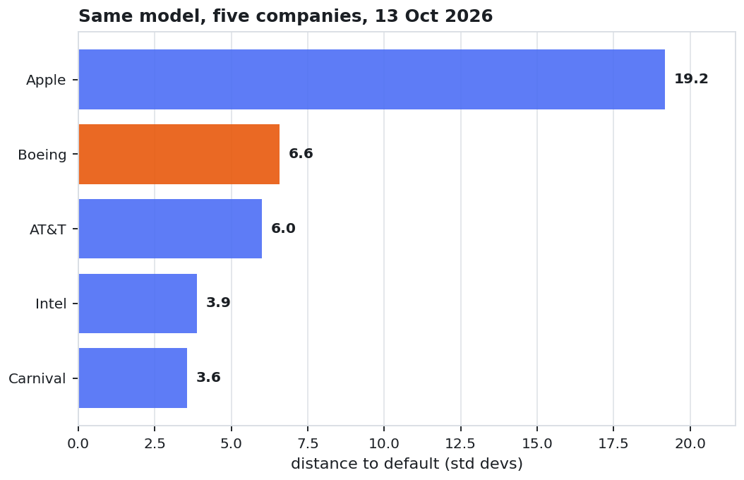
Boeing's shares are worth $147bn and swing 34% a year, against a default point of $25bn: debt due within a year plus half the rest, the KMV convention. Solving the two Merton equations backs out $172bn of assets at 29% vol, 6.6 standard deviations from default. In November 2020, with debt more than doubled and the Covid crash inside its one year vol, it was 1.75.

Solving Merton's two equations

def solve(E, sE, D, r, T=1.0):
    """Asset value and asset vol from equity value and equity vol."""
    def gap(z):
        V, sV = z
        d1 = (np.log(V / D) + (r + sV**2 / 2) * T) / (sV * np.sqrt(T))
        d2 = d1 - sV * np.sqrt(T)
        return [(V * norm.cdf(d1) - D * np.exp(-r * T) * norm.cdf(d2) - E) / E,
                (norm.cdf(d1) * sV * V - sE * E) / E]
    V, sV = fsolve(gap, [E + D, sE * E / (E + D)])
    dd = (np.log(V / D) + (r - sV**2 / 2) * T) / (sV * np.sqrt(T))
    return V, sV, dd

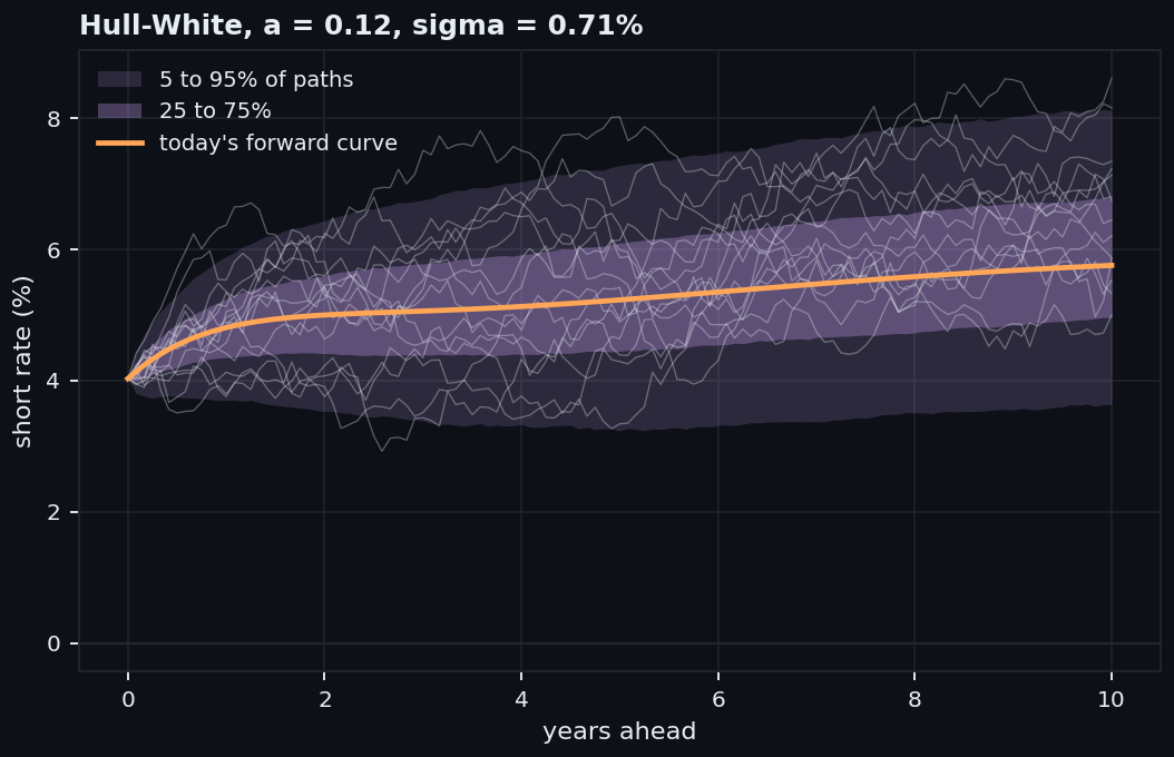
D = debt_short + 0.5 * debt_long          # KMV default point

5. Hull-White short rate model

Hull-White treats the short rate like a spring. It reverts at speed a toward a target path, fitted so today's curve comes out exactly, while shocks of size sigma push it around. Rates are normally distributed, which gives closed forms for bond options, caps and swaptions.

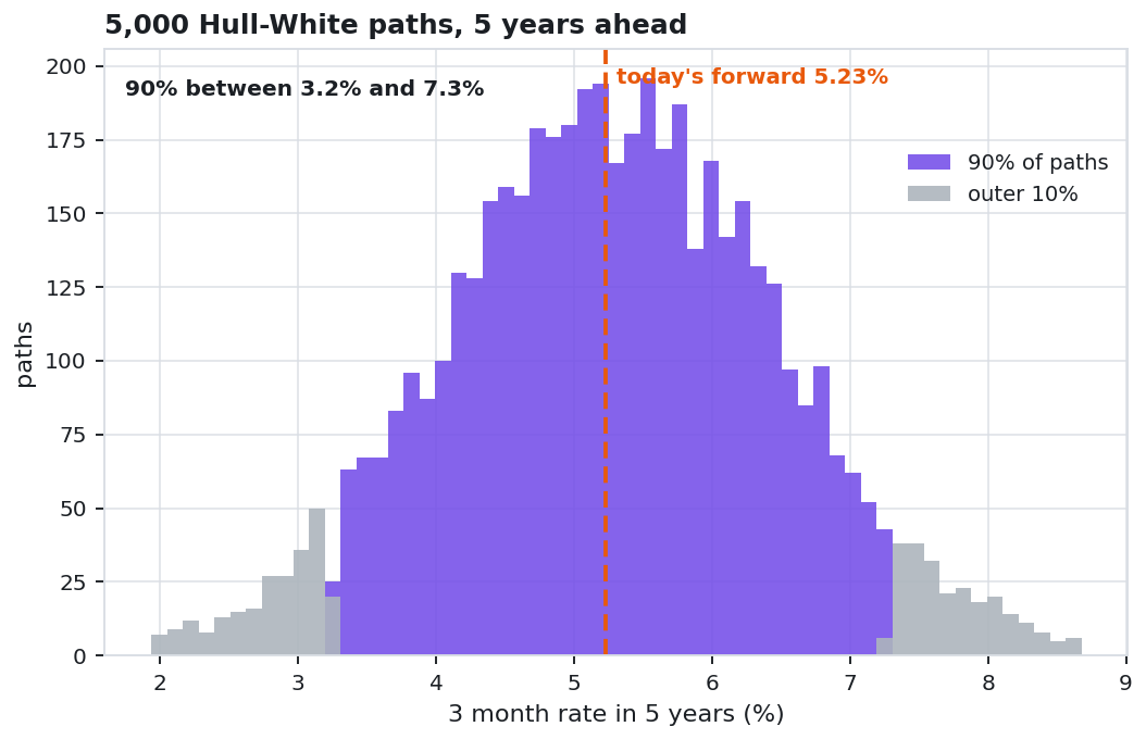
Fitted on month end 3 month T-bill yields since 1990, a comes out at 0.12, a half life of 5.8 years for any shock, and sigma at 0.71% a year. On 5,000 exact paths the model reprices the 5 year Treasury zero within 0.5 bp, and 90% of paths put the 3 month rate between 3.2% and 7.3% five years out.

Calibration and exact simulation

# a and sigma from an AR(1) on month end 3 month T-bill yields
phi, c0 = np.polyfit(bills[:-1], bills[1:], 1)
a = -np.log(phi) * 12
sigma = residuals.std() * np.sqrt(2 * a / (1 - np.exp(-2 * a / 12)))

# exact simulation: r = x + alpha, alpha puts the mean on today's forward curve
decay, sd = np.exp(-a * dt), sigma * np.sqrt((1 - np.exp(-2 * a * dt)) / (2 * a))
for i in range(steps):
    x[:, i + 1] = x[:, i] * decay + sd * rng.standard_normal(N)
alpha = f0 + sigma**2 / (2 * a**2) * (1 - np.exp(-a * t))**2
r = x + alpha

Run it

Full code in the repository: one file per model, the Treasury curve, the data loaders and the script that writes every chart and number. Data is cut at 2026-10-13, so a run on a later day gives the numbers on this page.

Clone and run

git clone https://github.com/davidalmeida90/quant-models
cd quant-models/fixed-income-options-models
pip install -r ../requirements.txt
export SEC_USER_AGENT="Your Name your@email"     # the SEC API asks for one
python run_all.py                                # charts/ and charts/facts.json

Limitations

• Historical vols. BDT and Hull-White take their vols from past yields (the 1 year, the 3 month bill, the 10 year), since swaption quotes are not free.
• Hypothetical convertible. The UBER bond on this page does not exist: 5 years, 1% coupon, 30% conversion premium.
• Pool priced at par. No free MBS prices exist, so the spread is set by pricing the pool at par. The page reports price changes and the option's value, which barely depend on that choice, and never the spread itself.
• Two Hull-White vols. The mortgage paths use sigma 1.15%, matched to the 10 year yield; the T-bill fit gives 0.71%, which moves the 10 year only about 40 bp a year.
• Simple prepayment rule. The S-curve has no burnout, seasonality or loan level data, and a dealer model would.
• Merton's distance. It uses the risk free drift and a one year horizon, and balance sheets enter at their period end, a month or so before they were filed.

Every run on one line

Related

• CRR binomial tree
• Yield curves, US and Brazil
• Volatility and option models
• Black-Scholes model
• Monte Carlo, GBM
• Machine learning for equity and fixed income