
Sell an at the money call, hedge it once a day with Black-Scholes delta, and simulate 150,000 price paths to see what a single day of hedging really costs. On the last day at the strike, one day of hedging noise is worth 76% of the option.
A delta hedge is meant to make an option position indifferent to small moves in the stock. In a textbook, rebalancing never stops and the risk disappears. On a real desk a hedge is adjusted at discrete moments, and between those moments the position still carries gamma. That leftover is the hedging error, and it is far from evenly spread.
Everything below comes from one short Python script. A call is sold exactly at the money with 20 trading days to expiry, implied volatility sits at 18%, and the price follows geometric Brownian motion drifting at a 2% risk-free rate, with realised volatility set equal to implied. That setup makes the hedge correct on average, so any profit or loss that appears is pure discretisation error, and gamma is what drives it.
Step by step, the page builds:
Only numpy, scipy and matplotlib are needed, and the full script runs in about ten seconds. Read the limitations before quoting a number here. There are no transaction costs, no jumps, volatility is constant and the interest rate is a flat 2%.
Gamma is the second derivative of the option price with respect to spot. This video goes past it, into vanna, volga, zomma, color and speed on a live NVDA option chain, with every closed form checked against a numerical derivative of the price surface before a single number is trusted. Zomma and speed describe exactly how the gamma measured on this page moves when volatility or spot change. Script and numbers for that one sit on the advanced greeks page.
I post the models as I build them, the changes I make to them, and the results that did not work. Shorter than these write ups, and there are a lot more of them.
Follow me on X


Sections below walk through the Monte Carlo step by step, with the reasoning, the charts and the code that matters. Full script, every figure it produces and the results file sit in the repository.
Short one call and hold delta shares against it. Rebalance at the start of the day and leave the position alone until the next morning. Over that day the book makes the change in the hedge minus the change in the option, plus one day of interest on the cash account. Buying delta shares costs more than the premium brings in, so that balance is negative and the interest is a cost:
P&L = Δ (S1 − S0) − (C1 − C0) + r Δt (C0 − Δ S0)Expanding the option price to second order shows where the money goes. Delta cancels by construction, interest on the cash cancels the part of theta that comes from the rate, and what survives is gamma against the size of the move:
P&L ≈ ½ Γ S² ( σ² Δt − (ΔS / S)² )A quiet day, with a move smaller than one expected daily standard deviation, leaves the book ahead: it collects the time decay. A large move in either direction costs money, and that loss grows with the square of the move. Both sides are multiplied by gamma, so wherever gamma is large the day swings hard, and wherever gamma is close to zero the hedge is close to perfect.
Three functions carry the whole model. Price values the call, delta sets the number of shares held, and gamma is only used to explain the results. Parameters sit at the top of the script so a single edit changes volatility, the rate, the option's life or the number of paths.
parameters
SIGMA = 0.18            # implied vol, and realised vol, annualised
S0 = K = 100.0          # the call starts exactly at the money
R = 0.02                # flat risk-free rate: prices drift at it and the hedge's cash pays it
DT = 1 / 252            # one trading day
LIFE_DAYS = 20          # the option is sold 20 trading days before expiry
N_PATHS = 150_000
SEED = 11
black_scholes.py
def d1(S, K, T, sig):
    return (np.log(S / K) + (R + 0.5 * sig ** 2) * T) / (sig * np.sqrt(T))


def call_price(S, K, T, sig):
    a = d1(S, K, T, sig)
    return S * norm.cdf(a) - K * np.exp(-R * T) * norm.cdf(a - sig * np.sqrt(T))


def call_delta(S, K, T, sig):
    return norm.cdf(d1(S, K, T, sig))


def gamma(S, K, T, sig):
    return norm.pdf(d1(S, K, T, sig)) / (S * sig * np.sqrt(T))
Two independent draws per path do the work. Z1 decides where spot has wandered by
the morning in question, and Z2 decides the move during that day. Both are drawn once
and reused at every maturity, a technique called common random numbers. Comparing 10 days to
expiry with 1 day therefore compares time and nothing else, because the randomness underneath
is identical.
Prices drift at the risk-free rate and realised volatility equals implied volatility, so the hedge is right on average. Any profit or loss that appears below is discretisation error, meaning the price of adjusting the hedge once a day instead of continuously.
one_day_of_hedging.py
rng = np.random.default_rng(SEED)
Z1 = rng.standard_normal(N_PATHS)      # where spot has wandered to by the start of the day
Z2 = rng.standard_normal(N_PATHS)      # the move during that one day


def one_day_of_hedging(tau_days):
    """P&L of a short call hedged with delta shares over one day, starting tau_days before expiry.

    Z1 and Z2 are reused for every tau, common random numbers, so results at different
    maturities differ because of time and nothing else. Buying delta shares uses more cash than
    the premium brings in, so the cash balance is negative and pays interest over the day.
    """
    elapsed = (LIFE_DAYS - tau_days) * DT
    s = S0 * np.exp((R - 0.5 * SIGMA ** 2) * elapsed + SIGMA * np.sqrt(elapsed) * Z1)
    s_next = s * np.exp((R - 0.5 * SIGMA ** 2) * DT + SIGMA * np.sqrt(DT) * Z2)
    t0, t1 = tau_days * DT, (tau_days - 1) * DT
    c0 = call_price(s, K, t0, SIGMA)
    c1 = np.maximum(s_next - K, 0.0) if t1 <= 1e-9 else call_price(s_next, K, t1, SIGMA)
    hedge = call_delta(s, K, t0, SIGMA)
    cash = c0 - hedge * s                              # premium in, shares bought, negative
    pnl = -(c1 - c0) + hedge * (s_next - s) + cash * np.expm1(R * DT)
return s / K, pnlEvery dot is one path: where spot sat relative to the strike that morning, and what the hedged position made or lost by the next one. Ten trading days before expiry the cloud is a wide, flat band. On the last day it collapses into a sharp shape centred on the strike.
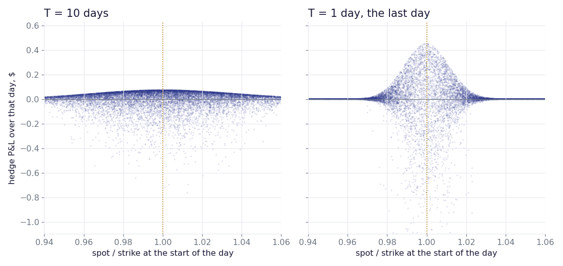
Two features give the shape away. Gains have a hard ceiling: if spot does not move at all, the best a short option can do is keep one day of time value, less a day of interest on the hedge. Losses have no floor, since a large move costs gamma times its square. Both are measured below against theory.
| Days to expiry | Best day, simulated | Ceiling, theory | Worst day | Average day |
|---|---|---|---|---|
| T = 10 days | $0.0734 | $0.0734 | −$1.56 | +0.0004 |
| T = 5 days | $0.1068 | $0.1067 | −$1.79 | +0.0003 |
| T = 2 days | $0.1874 | $0.1873 | −$2.17 | +0.0002 |
| T = 1 day | $0.4521 | $0.4523 | −$2.66 | +0.0001 |
Simulated ceilings land within 0.0003 of theory at every maturity, which is the check that the engine is doing what the formula says. On the last day the ceiling reaches $0.45, nearly the entire remaining value of the option, because a call worth $0.46 that finishes exactly at the strike expires worthless, and only a day of interest on the hedge comes off. Average P&L stays at zero throughout, as it should when realised and implied volatility are equal. Worst days deepen from −$1.56 to −$2.66 as expiry approaches.
A scatter shows the shape. A number needs the spread. Paths are grouped by where spot started the
day relative to the strike, and the standard deviation of one day's P&L is taken inside each
group. np.bincount does it without a Python loop, which matters at 150,000 paths.
Groups with fewer than 900 paths are left blank so that thin tails do not draw false spikes.
spread_by_moneyness.py
EDGES = np.linspace(0.94, 1.06, 49)
CENTRES = (EDGES[:-1] + EDGES[1:]) / 2
AT_STRIKE = int(np.argmin(np.abs(CENTRES - 1.0)))


def spread_by_moneyness(m, pnl, min_count=900):
    idx = np.digitize(m, EDGES) - 1
    ok = (idx >= 0) & (idx < len(CENTRES))
    n = np.bincount(idx[ok], minlength=len(CENTRES)).astype(float)
    s1 = np.bincount(idx[ok], weights=pnl[ok], minlength=len(CENTRES))
    s2 = np.bincount(idx[ok], weights=pnl[ok] ** 2, minlength=len(CENTRES))
    with np.errstate(invalid="ignore", divide="ignore"):
        std = np.sqrt(np.maximum(s2 / n - (s1 / n) ** 2, 0.0))
    std[n < min_count] = np.nan
    return std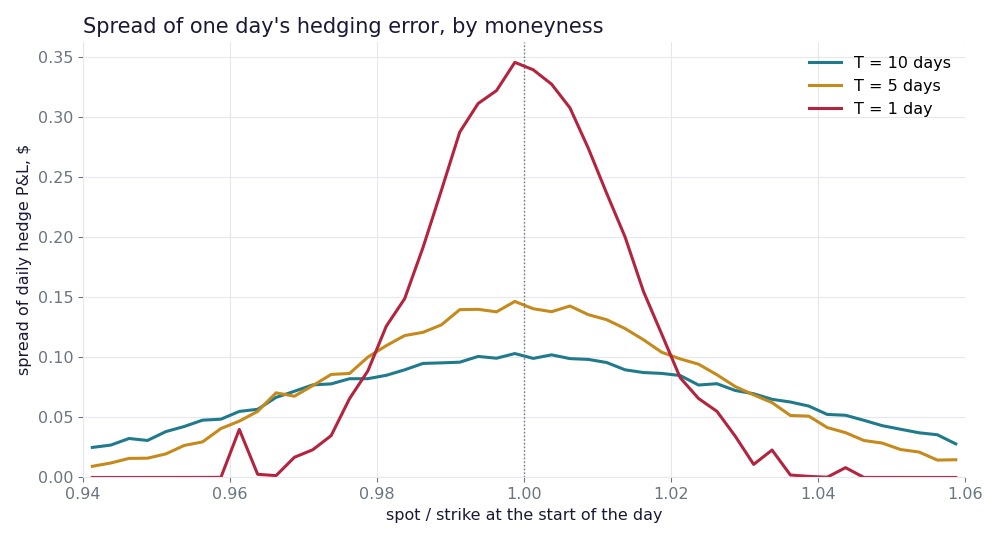
| Days to expiry | Gamma | Spread of daily P&L | Multiple of T = 10 |
|---|---|---|---|
| T = 10 days | 0.1112 | $0.103 | 1.00x |
| T = 5 days | 0.1573 | $0.147 | 1.42x |
| T = 2 days | 0.2487 | $0.232 | 2.25x |
| T = 1 day | 0.3518 | $0.346 | 3.35x |
At the strike, the spread grows 3.4 times between 10 days and the last day. Square root of time predicts 3.16 times, because gamma scales with one over the square root of time to expiry. Simulation lands slightly above that on the final day, where a one day step equals the whole remaining life of the option and the small step approximation behind the square root rule stops holding. Five percent away from the strike on that same day, the spread falls to 0.0000015: gamma is essentially zero there, and a delta hedge is essentially perfect.
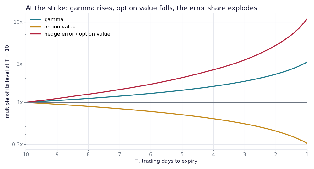
$0.346 on its own says little. Measured against what the option is actually worth, it becomes the most important number on the page. Three things move at the strike as expiry approaches, and they move in opposite directions.
| Days to expiry | Option value | Daily hedge error | Error / value |
|---|---|---|---|
| T = 10 days | $1.47 | $0.103 | 7.0% |
| T = 5 days | $1.03 | $0.147 | 14.2% |
| T = 2 days | $0.65 | $0.232 | 35.8% |
| T = 1 day | $0.46 | $0.346 | 75.8% |
Gamma rises by the square root of ten, 3.16 times, while the option's value falls by about the same factor, to 0.31 of where it started. Hedge error follows gamma, so its share of the option grows by roughly ten times, from 7% of the premium to 76%. One day of ordinary hedging noise on the last day is worth three quarters of everything the option still carries.
That share does not depend on the level of volatility. Error scales with gamma times volatility squared, gamma scales with one over volatility, and the option's value scales with volatility, so volatility cancels. Only the ratio of the hedging interval to the time left matters, which is why the last day is so much worse than any other.
If gamma is the problem, frequency is the tool. Splitting the final day into N rebalances shrinks each move between adjustments, and the spread of P&L falls with the square root of N. Each path below starts the last morning exactly at the strike, which is the worst place to be.
last_day_rebalanced.py
def last_day_rebalanced(n_rebalances, paths=200_000, seed=3):
    """Final day only, spot opening exactly at the strike, delta rebalanced n times in the day."""
    g = np.random.default_rng(seed)
    h = DT / n_rebalances
    s = np.full(paths, K)
    cash = np.full(paths, float(call_price(K, K, DT, SIGMA)))     # premium received
    shares = np.zeros(paths)
    for i in range(n_rebalances):
        hedge = call_delta(s, K, DT - i * h, SIGMA)
        cash -= (hedge - shares) * s                               # buy or sell the difference
        shares = hedge
        s = s * np.exp((R - 0.5 * SIGMA ** 2) * h + SIGMA * np.sqrt(h) * g.standard_normal(paths))
        cash *= np.exp(R * h)                                      # interest until the next rebalance
    pnl = cash + shares * s - np.maximum(s - K, 0.0)               # close the book at expiry
    return float(pnl.std()), float(pnl.mean())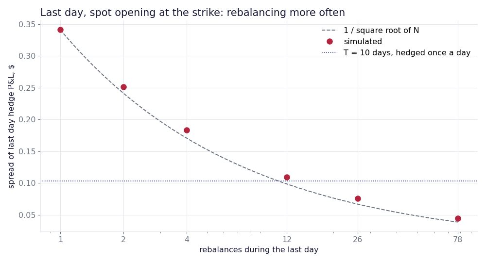
| Rebalances | Every | Spread of P&L | Reduction |
|---|---|---|---|
| 1 | 390 min | $0.341 | 1.0x |
| 2 | 195 min | $0.251 | 1.4x |
| 4 | 98 min | $0.184 | 1.9x |
| 12 | 32 min | $0.110 | 3.1x |
| 26 | 15 min | $0.076 | 4.5x |
| 78 | 5 min | $0.044 | 7.7x |
Matching the accuracy that one rebalance a day delivered at 10 days to expiry takes 12 rebalances on the last day, roughly every 32 minutes, which brings the spread to $0.110. Every five minutes cuts it to $0.044. Simulation follows the one over square root of N rule closely at every step.
That is exactly the trade a market maker lives with. Every rebalance crosses a bid ask spread, and at the strike on expiry day delta swings the most, so the hedge needs the most adjustments precisely where each adjustment costs the most. Holding gamma into the close means choosing between hedging noise and transaction costs, and neither one goes away.
| Days to expiry | Option value | Gamma | Daily hedge error | Error / value |
|---|---|---|---|---|
| T = 10 days | $1.47 | 0.1112 | $0.103 | 7.0% |
| T = 5 days | $1.03 | 0.1573 | $0.147 | 14.2% |
| T = 2 days | $0.65 | 0.2487 | $0.232 | 35.8% |
| T = 1 day | $0.46 | 0.3518 | $0.346 | 75.8% |
Delta hedging works best where it is needed least. Away from the strike, or with plenty of time left, one rebalance a day leaves a small and predictable error. At the strike in the final days, gamma rises while the option shrinks, and a hedge that looked adequate a week earlier becomes noise worth most of the premium. Rebalancing more often buys it back, at a cost that grows in the same place.